Aggregate Demand and Aggregate Supply

Short-Run Economic Fluctuations

• Economic activity varies from year to year.

• In the short run, GDP oscillates around its trend.

  • Most years see an increase in the production of goods and services.

  • Recessions occur when normal growth is disrupted.

    • Recession: A period marked by declining real incomes and increasing unemployment.

    • Depression: A severe and rare form of recession.

• Short-run economic fluctuations are often referred to as business cycles, representing the natural rise and fall of economic growth over time.

Three Facts About Economic Fluctuations

• FACT 1: Economic fluctuations are irregular and unpredictable

• FACT 2: Most macroeconomic variables fluctuate together, however they fluctuate by different amounts

• FACT 3: As output rises, unemployment falls

Explaining Short Run Economic Fluctuation

• The theory of economic fluctuations is complex and contentious.

• Most economists utilize the aggregate demand and aggregate supply model to analyze these fluctuations.

• This model contrasts with classical economic theories used for long-run analysis.

The Basic Model of Economic Fluctuations

• Two variables used to develop a model

  • The economy’s output of g&s measured by real GDP

  • The overall price level measured by CPI/GDP deflator

  => The model of AS - AD

• The economy’s output of goods and services, measured by Y.

• The overall price level, measured by P.

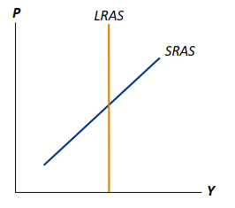
• Model of Aggregate Demand and Aggregate Supply:

  

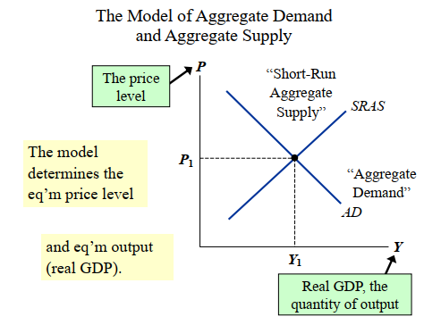
  • The model determines the equilibrium price level and equilibrium output (real GDP - many kinds of output).

  • AD represents "Aggregate Demand."

  • SRAS represents "Short-Run Aggregate Supply."

    • Reminder: SRAS is short-run because in the long run, supply curve is vertical

    • Long-run output (Y) does not depend on price PPF

The Aggregate-Demand (AD) Curve

• The AD curve illustrates the quantity of all goods and services demanded in the economy at any given price level.

  

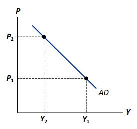
Why the AD Curve Slopes Downward

• The four components of GDP (Y) contribute to the aggregate demand for goods and services.

• AD = C + I + G + NX

  • This equals to GDP, but different from GDP

  • GDP is actual expenditure, while AD is planned expenditure, but based on current price level and demand

• Assume G is fixed by government policy (exogenous).

• To understand the slope of AD, we must determine how a change in P affects C, I, and NX.

The Wealth Effect (P and C)

• Mechanism:

  • P falls → real value of money falls → C falls → AD falls

  • P rises → real value of money rises → C rises → AD rises

  • A lower price level increases the real value of money holdings (cash, bank accounts). Consumers feel wealthier and spend more on goods and services.

• Example:
  If P falls by 20%, the same amount of money buys 20% more goods. Households increase consumption (C).

• Effect on AD:
  Lower P → Higher real wealth → Higher C → Increased quantity of output demanded (Y).

The Interest-Rate Effect (P and I)

• Mechanism:

  • P rises → demand for money rises (more money is needed for transactions now that things become more expensive) → deposit less money in banks → higher interest rates → discouraged borrowing for investment

  • A lower price level reduces the demand for money (since less money is needed for transactions). People lend excess money (e.g., buy bonds), lowering interest rates (r). Lower r encourages borrowing for investment (I) and big-ticket consumer purchases.

• Example:
  If P falls, households deposit more money in banks → banks lower interest rates → firms borrow more to build factories.

• Effect on AD:
  Lower P → Lower r → Higher I and C → Increased Y.

The Exchange-Rate Effect (P and NX)

• Mechanism:

  • P rises → demand for money rises → people lend less, sell bonds and hold more money → higher interest rates

  • Higher domestic interest rates attract investors → Foreigners buy domestic assets (US bonds) → increasing demand for domestic currency → domestic currency appreciates

  • A stronger currency makes exports more expensive for foreigners and imports cheaper for domestic buyers → X falls, M rises → NX falls

  • A lower price level reduces interest rates (r), making domestic assets less attractive. Investors sell domestic currency to buy foreign assets → domestic currency depreciates. Cheaper domestic goods boost exports (XX), while foreign goods become more expensive, reducing imports (MM). Net exports (NX=X−M) rise.

• Example:
  Lower P in the U.S. → Lower U.S. interest rates → Dollar depreciates vs. euro → U.S. goods cheaper for Europeans → U.S. exports increase.

• Effect on AD:
  Lower P → Lower r → Currency depreciation → Higher NX → Increased Y.

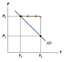
The Slope of the AD Curve: Summary

• An increase in P reduces the quantity of goods and services demanded due to:

  • The wealth effect (P rises → C falls)

  • The interest-rate effect (P rises → I falls)

  • The exchange-rate effect (P rises → NX falls)

Why the AD Curve Might Shift

• Any event that alters C, I, G, or NX (excluding a change in P) will cause the AD curve to shift. (AD does not depend on P)

  

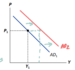
  • Changes in C

    • Stock market boom/crash (Household wealth rises/falls → AD shifts right/left)

    • Preferences: consumption/saving tradeoff (S rises → C falls → AD shifts left)

    • Tax hikes/cuts (Disposable income Y_d = Y - T = C + S ) => fiscal

  • Changes in I

    • Firms buying new computers, equipment, factories

    • Expectations, optimism/pessimism

    • Interest rates, monetary policy

    • Investment Tax Credit or other tax incentives

  • Changes in G

    • Central spending, e.g., defense

    • Local spending, e.g., roads, schools

  • Changes in NX

    • Booms/recessions in countries that buy our exports.

    • Appreciation/depreciation resulting from international speculation in the foreign exchange market.

The Aggregate-Supply (AS) Curves

• The AS curve shows the total quantity of goods and services firms produce and sell at any given price level.

  • AS is upward-sloping in the short run.

  • AS is vertical in the long run.

    

The Long-Run Aggregate-Supply Curve (LRAS)

• The natural rate of output (Y_N) is the amount of output the economy produces when unemployment is at its natural rate.

• Y_N is also called potential output or full-employment output.

  

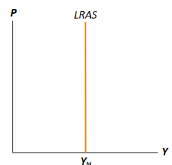
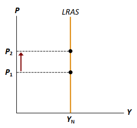
Why LRAS Is Vertical

• Y_N is determined by the economy’s stocks of labor, capital, and natural resources, and on the level of technology.

• An increase in P does not affect any of these, so it does not affect Y_N (Classical dichotomy).

  

Why the LRAS Curve Might Shift

• Any event that changes any of the determinants of Y_N will shift LRAS.

• Eg: Immigration rises → L rises → LRAS shifts right

  • Changes in L or the natural rate of unemployment

    • Immigration

    • Baby-boomers retiring

    • Government policies reducing the natural unemployment rate

  • Changes in K or H

    • Investment in factories, equipment

    • More people obtaining college degrees

    • Factories destroyed by a hurricane

  • Changes in natural resources

    • Discovery of new mineral deposits

  • Changes in technology

    • Productivity improvements from technological progress

Short Run Aggregate Supply (SRAS)

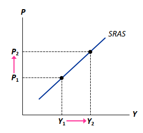
• The SRAS curve is upward sloping.

• Over a period of 1-2 years, an increase in P causes an increase in the quantity of goods and services supplied.

Three Theories of SRAS

• Each theory involves some type of market imperfection.

• Result: Output deviates from its natural rate when the actual price level deviates from the price level people expected.

Why the SRAS Curve Slopes Upward

Common element of all 3 theories

• Y deviates from Y_N when P deviates from P_E

  

• Y = Y_N + a(P – P^E)

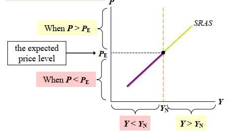
  • Y: Output

  • Y_N: Natural rate of output (long-run)

  • a > 0, measures how much Y responds to unexpected changes in P

  • P: Actual price level

  • P_E: Expected price level

The Sticky-Wage Theory

• Imperfection: Nominal wages are sticky in the short run, adjusting slowly due to labor contracts and social norms.

• Firms and workers set the nominal wage in advance based on P^E, the price level they expect.

• If P > P^E, revenue is higher, but labor cost is not. Production is more profitable, so firms increase output and employment.

• Hence, higher P causes higher Y, so the SRAS curve slopes upward.

The Sticky-Price Theory

• Imperfection: Many prices are sticky in the short run due to menu costs (the costs of adjusting prices).

• Firms set sticky prices in advance based on P^E.

• If the central bank increases the money supply unexpectedly, P will rise in the long run.

• In the short run:

  • Firms without menu costs can raise prices immediately.

  • Firms with menu costs wait to raise prices. Consequently, their prices are relatively low, increasing demand for their products, and they increase output and employment.

• Hence, higher P is associated with higher Y, so the SRAS curve slopes upward.

The Misperceptions Theory

• Imperfection: Firms may confuse changes in P with changes in the relative price of their products.

• If P rises above P^E, a firm sees its price rise before realizing all prices are rising. The firm may believe its relative price is rising and may increase output and employment.

• Thus, an increase in P can cause an increase in Y, making the SRAS curve upward-sloping.

SRAS vs. LRAS

• The imperfections in these theories are temporary. Over time:

  • Sticky wages and prices become flexible.

  • Misperceptions are corrected.

• In the long run:

  • P = P^E

  • AS curve is vertical

    

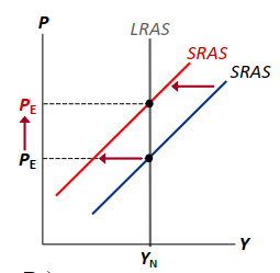
Why the SRAS Curve Might Shift

• Everything that shifts LRAS shifts SRAS, too.

• P^E shifts SRAS: If P^E rises, workers & firms set higher wages. At each P, production is less profitable, Y falls, and SRAS shifts left.

  

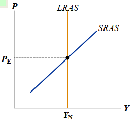
Equilibrium

• In the long-run equilibrium, P = P^E , Y = Y_N, and unemployment is at its natural rate.

• In the short-run equilibrium, SRAS intersects AD.

  

Analyzing Economic Fluctuations

• Caused by events that shift the AD and/or AS curves.

• Four steps to analyzing economic fluctuations:

  1. Determine whether the event shifts AD or AS.

  2. Determine whether the curve shifts left or right.

  3. Use the AD-AS diagram to see how the shift changes Y and P in the short run.

  4. Use the AD-AS diagram to see how the economy moves from the new SR equilibrium to the new LR equilibrium.

The Effects of a Shift in AD

• Event: Stock market crash

  1. Affect C → AD curve

  2. Crash → less wealth → C falls → AD shifts left

  3. Short run equilibrium at C

  4. P and Y lowers => Unemployment higher

  

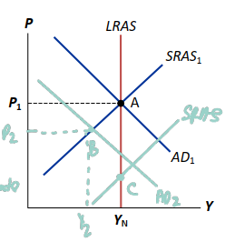
• In the long run, unemployment rate > natural rate → Firms hold power → Wages fall → SRAS shifts to the right, eventually restoring full employment as the economy adjusts at initial levels

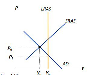
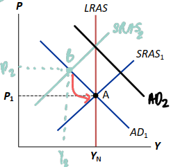
The Effects of a Shift in SRAS

• Event: Oil prices rise

  1. Rising production costs → Affect SRAS curve

  2. Firms supply less output → SRAS shifts left

  3. Short run equilibrium at B. P higher, Y lower, unemployment higher

  4. From A to B, stagflation a period of falling output and rising prices

John Maynard Keynes

• (1883-1946)

• Argued recessions and depressions can result from inadequate demand; policymakers should shift AD.

• Famous critique of classical theory:

  • Economists set themselves too easy, too useless a task if in tempestuous seasons they can only tell us when the storm is long past, the ocean will be flat.

  • "The long run is a misleading guide to current affairs. In the long run, we are all dead."

  • “time will heal all wounds” ???

Conclusion

• This chapter introduced the model of aggregate demand and aggregate supply, which helps explain economic fluctuations.

• Keep in mind: these fluctuations are deviations from long-run trends

• In the next chapter, we will learn how policymakers can affect aggregate demand with fiscal and monetary policy.