AP STATS CRAM REVIEW
Unit 1: Exploring One-Variable Data
DESMOS GUIDES:
categorical variable: takes on names or labels
ex: eye color, marital status, etc
categorized in two-way table (two variables)

marginal relative frequency = total in single row or column / final total
ex: 10 (math total) / 23 (total)
joint relative frequency = single number / final total
ex: 3 (math + internal) / 23 (total)
conditional relative frequency = single number / total in associated row or column
ex: 3 (math + internal) / 10 (math total)
quantitative variable: takes on numeric values
discrete variables (1, 2, 3, 4)
continuous variables (5’4, 5’11, decimals)
how to describe variable (CSOCS)
Context
Shape (symmetrical, skewed, # of peaks)
unimodal (one peak), bimodal (2 peaks)
uniform or skewed left/right distributions
Outliers
Center (mean/median)
Spread (range, standard deviation, interquartile range)
use descriptive and comparitive language (similarly, roughly)
important terms
mean = sum of values / # of values
standard deviation
"[value] typically varies by [SD] from the mean of [mean]”
SD² = variance
z-score (# of standard deviations a value is away from the mean) = (value - mean) / SD
median = middle value when organized least to greatest
50th percentile
range = max - min
interquartile range (IQR) = Q3 (75th percentile) - Q1 (25th percentile)
box plot points: minimum → Q1 → median → Q3 → maximum

outliers
low-end outlier (super low outlier) < Q1 - (1.5 * IQR)
high-end outlier (super high outlier) > Q3 + (1.5 * IQR)
2 SD away from the mean (z-score) → outlier
percentile = % of values less than/equal to a specific value
cumulative relative frequency = shows cumulative percentages from each interval
chance of something happening

transforming the data
add/subtract all data by same amount
shape + variability stay the same
center moves up/down by that amount
multiply/divide all data by same amount
shape stays the same
center + variability multiplied/divided by that amount
normal distributions
type of density curve (shows probability distribution, total area of 1)

68% of values = within 1 SD
95% of values = within 2 SD
99.7% of values = within 3 SD
calculator functions
normPdf = probability of specific value
normCdf = probability that variable is between set interval
invNorm = find value that corresponds with percentile
normal probability distribution (shows how well the data fits normal distribution)
plots actual values vs. theoretical z-values (normally distributed)
roughly linear = roughly normal distribution
non-linear = not roughly normal distribution
Unit 2: Exploring Two-Variable Data
to describe scatterplots (CDOFS)
Context
Direction (+/-)
Outliers
Form (linear/nonlinear)
Strength (weak, moderate, strong)
r value = correlation coefficient
closer to -/+ 1 = stronger linear correlation
EX: -0.97 = strong negative, 0 = no correlation, 0.021 = weak
changing units or switching axes → doesn’t affect R
outliers can change R

outliers within “pattern of data” → strengthens R
outliers outside “pattern of data” → weakens R
regression line = line of best fit (estimates values not given)
equation: y (hat) = a + bx
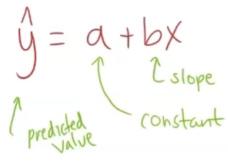
y (hat) = PREDICTED y-value, not actual
a = constant
b = slope
residual = degree of error of regression line prediction
equation: y - y(hat) = residual
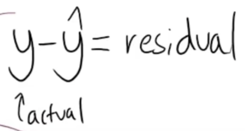
negative = residual line overestimated (greater than) actual values
positive = residual line underestimated (lower than) actual values
HOW TO INTERPRET

least squares regression line (LSRL) = line that minimizes sum of square residuals (aka kinda best fit line)
plug big dataset into calculator → LSRL
key LSRL values
s value = avg distance predicted values are form the LSRL
r² value = coefficient of determination (% of response variables that are explained by explanatory variable)
lower s + higher r² = better LSRL
outliers
outliers added far away from the mean of y
DECREASE in slope + INCREASE in y-intercept
outliers added above mean of x
slope is unchanged, DECREASE in y - intercept
outliers added below mean of x
slope is unchanged, INCREASE in y - intercept
residual plots (shows residual values vs explanatory variable)
clear pattern = linear function is not likely best fit for data

unclear pattern = linear function is likely best fit for data
Unit 3: Collecting Data
random sampling methods
simple random sample (SRS) = randomly selected subset population
all numbers in sample has equal chance of being selected
process:
define population → label individuals (number, names on paper, etc)
randomize (random # generator, names in hate, etc)
select members of randomized sample
stratified random sample = split population into groups (strata) of shared traits → randomly select samples
EX: divide school by grade level → randomly picking a student from each grade
groups are homogeneous
cluster sample: splits population into groups → randomly select ENTIRE CLUSTERS to sample
EX: splitting city into neighborhoods → surveying EVERYONE in randomly chosen NEIGHBORHOODS
groups are heterogeneous
systematic random sample: select individuals at regular set intervals
EX: picking every 5th person on a class roster and starting at a random number (5th, 10th, 15th, etc)
BAD common sampling methods
convenience sampling = choosing people who are easy to reach
EX: surveying people at nearby mall cus it’s closest
voluntary response sampling = allowing people to choose to participate
EX: online poll where only people who feel strongly respond
shortcomings to collecting data
undercoverage = some groups are left out and underrepresented
EX: survey sent out to people with internet access → those who don’t have internet are left out
nonresponse = individuals don’t/can’t respond
response bias = people giving false/misleading answers
EX: lying about exercising to seem like they are healthier
poor wording to a question → influenced answers
EX: “would you do this to get 1 million dollars?”
observational study = observe/collect data without influencing subjects
experiment = manipulating variables/applying treatments to observe/measure effects on subjects
4 principles of experimental design
comparison (compare 2+ groups to see difference in treatment)
random assignment (randomly assign subjects to groups to reduce bias)
control (keep variables constant
replication (use a good amount of subjects and repeat treatments)
key terms:
factor = explanatory variable or independent variable
EX: sunlight
level = value/category of the factor
EX: low/high sunlight
confounding = when another variable affects results
hard to tell which is the true cause
placebo = fake treatment
to see if participants may act favorably to it because they THINK its the real treatment
single-blind = subjects don’t know what group they’re in + researchers know
double-blind = subjects + researchers don’t know what group is getting what treatment
Unit 4: Probability, Random Variables, and Probability Distributions
probability = chance that event will happen written as number between 0 and 1
unpredictable in short term, predictable in long-term
need to observe a lot of trials so that random chance can approach its actual probability
simulation = model used to mimic real-world events to estimate probabilities
process:
state (define problem/question)
plan (describe how to use a chance device to model the situation)
do (preform multiple trials of simulation)
conclude (use results to estimate probability)
probability terms:
mutually exclusive = two events that don’t overlap + can’t occur at the same time

independent = outcome of one event doesn’t affect the outcome of the other
EX: rolling die and flipping a coin
probability rules (ON AP EXAM REFERENCE SHEET):

probability of EITHER event A/B happening
probability of non mutually exclusive events (can happen at the same time) = (prob A + prob B) - overlap
probability of mutually exclusive events (canNOT happen at the same time) = prob A + prob B

probability of BOTH occuring
non independent (A affects B) = prob B * prob A after prob B has happened OR prob A * prob B after A has happened
prob A after B has happened (P(A|B)) = overlap / prob B

independent = prob A * prob B
probability of A not occurring = 1 - prob A
same with prob B
types of probability visualization
probability tree

venn diagram

two way table

random variables
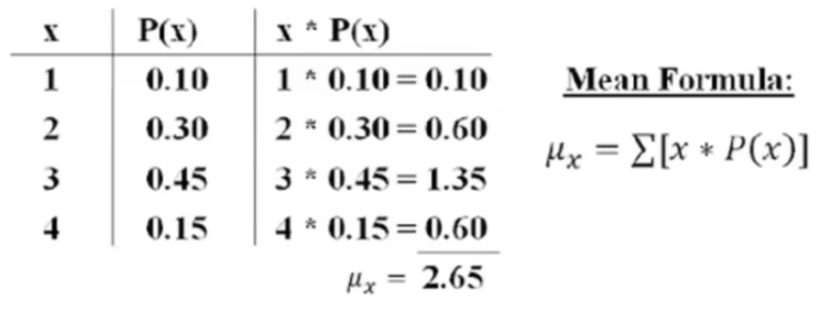
discrete random variable = takes on specific, countable values
calculate mean/expected value = (prob x1 * x1) + (prob x2 * x2) + etc…etc…
continuous random variable = can take on any value within a range/interval (included decimals)
binomial random variables = several independent trials of same chance process → record # of times that particular outcome occurs
requirements (BINS)
Binary? (success vs failure)
Independent? (trial outcome doesn’t affect other outcomes)
Number? (number of trials (n) should be fixed)
Success? (probability (p) must be set)
mean/SD equations (ON REFERENCE SHEET)

commands on calculator:
BinomPdf = (n, p, x)
n = # of trials
p = probability
x = # of successes out of trials
BinomCdf = (n, p, lower, upper)
cumulative probability
geometric random variables = models # of trials required to achieve first success in a series of independent trials
no fixed # of trials
mean/SD equations (ON REFERENCE SHEET)

commands on calculator
GeometricPdf = computes probability that first success happens on a specific trial
GeometricCdf = computers probability that first success happens between range of trials
transforming probability distributions
adding/subtracting by same number (constant = c) to each #
shape + variability = unchanged
center = increases/decreases by c
multiplying/dividing same number (c) to each #
shape = unchanged
center + variability = multiplied/divided by c
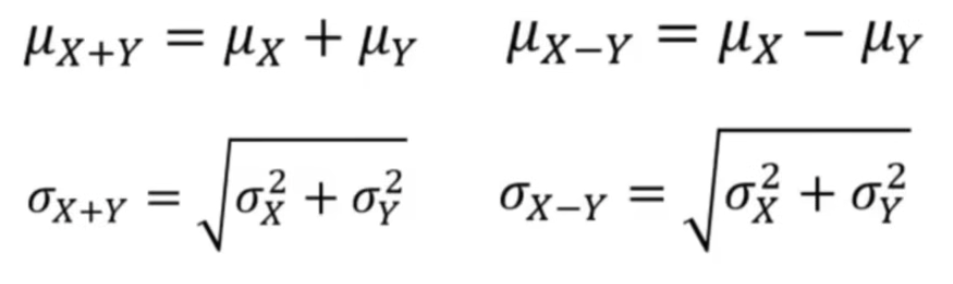
adding/subtracting independent random variables
Unit 5: Sampling Distributions
statistic = measure computed from sample of data
parameter = measure computed from entire population of data
notations

sampling distribution = probability distribution of a statistic obtained through repeated sampling of specific population

unbiased estimator: mean of statistic’s sampling distribution = parameter
sampling distributions for proportions
steps:
take repeated samples of same size from population
find proportion of outcome of each sample
plot proportions onto distribution
mean/SD (ON REFERENCE SHEET)
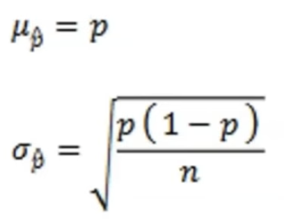
increasing sample size → decreases variability of distribution
needed assumptions:
random sampling/assignment
10% condition = sample size needs to be less than/equal to 10% of population size
allows trials to be treated as independent
representation → n < 0.1N
large counts condition = expected # of successes and failures is greater than or equal to 10 → sampling distribution is normal
representation → np 10 or n (1 - p) 10
if normal → can find z-value (how many SD away from the mean)

can find probability by using NormCdf
sampling distributions for means
steps:
take repeated samples of same size from population
find means of outcome of each sample
plot means onto distribution
mean/SD (ON REFERENCE SHEET)

increasing sample size → decreasing variability
assumptions needed
random sampling
10% condition
large counts condition
z-value for means (ON REFERENCE SHEET)

sampling distribution sample size is at least 30 → distribution is normal (central limit theorem)
?? Unit 6: Inference for Proportions
point estimate: value (statistic) to estimate population parameter
confidence interval: range of values to estimate population parameter
interp: “we are [confidence]% confident that the interval from [min] to [max] captures the true [parameter in context]”
basically the conclusion
testing confidence intervals (PANIC)
Parameter of interest (proportion of [context])
Assumptions (conditions)
random sample
independent (if n is less than/equal to 10% of population)
normal if sample proportion (p hat) is greater than or equal to 10
check for both in two sample datasets
Name of the test
Intervals

Conclusion
within context (using interpretation)
(for two sample) if interval includes 0 (ex: -3.2 < x < 1.0) → cannot conclude difference in population proportions
confidence level: probability that parameter falls within a specified range
interp: “if we make many, many [confidence intervals] we ca expect about [confidence level] % of the intervals to capture the true [parameter in context]”
increase → increase in margin of error (wider)
increase sample size → decrease margin of error (narrower)
bias DOES NOT affect margin of error
significance tests for proportions (PHANTOMS)
Parameter of interest
Hypothesis
Ho = null hypothesis
always should be described with =
Ha = alternate hypothesis
usually greater than, less than, unequal to
what we’re finding evidence for
Assumptions/conditions
Name of test (which is the significance test)
Test statistic (calculate with calculator, not by hand)
Obtain p-value (determines if you reject/fail to reject null hypothesis)
0.05 = alpha value (probability of rejecting Ho when Ha is true)
if p < 0.05 → reject null hypothesis
if above → not significant enough to reject
Make decision (reject or fail to reject Ho)
State conclusion in context
mention Ha in context

type 1 error = null hypothesis is true, but its rejected and we conclude Ha
false negative
alpha value = probability of making type 1 error
type 2 error = null hypothesis is false, but we fail to reject it and can’t conclude Ha
power: probability that a false Ho will be rejected when Ha is true
equation = 1 - probability of making a type 2 error or P(type 2 error)
to increase power
increase alpha value (will increase chance of type 1 error)
increase sample size
increase distance between Ho/Ha (will cause test to be more sensitive to significant differences)
Unit 7: Inference for Means
degrees of freedom (df) = # of values in data that can vary freely without affecting others
for significance tests/confidence intervals for means → df = n - 1
needed to calculate t* (instead of z* from unit 6)
confidence intervals for means
define parameters (use in context)
name the procedure (one or two sample t-interval)
conditions/assumptions
random sample
independent if sample is less than or equal to 10% of population
normal if (satisfy one of three conditions)
population is normal (stated)
CLT (sample size is greater than/equal to 30)
sample doesn’t have strong skewness/outliers
interpretation
“we are [percent]% confident that the interval from [interval to interval] captures the true mean of…”
2 sample = same thing but its “difference in means” at the end
significance test for means
write hypotheses + define parameters
find Ho (null) and Ha (alternative)
find true mean of….
name the procedure (one sample/two sample t-test for mean)
assumptions/conditions
random sample
independent if n is less than or equal to 10% of N
normal if (one of these conditions should be met)
population = normal
n is greater than or equal to 30 (CLT)
sample shows no strong skewness/outliers
interpretation
if p-value is less than/equal to alpha value (0.05) → reject Ho → “we have convincing evidence that the true mean of [Ha]
if p-value is greater than alpha value (0.05) → fail to reject Ho → “we do not have convincing evidence that the true mean of [Ha]
Unit 8: Inference for Chi-Square
chi-squared test for goodness of fit
“does a sample’s observed distribution significantly differ from the expected distribution?”
there is no parameter + sample statistic
steps
find hypotheses (Ho + Ha)
assumptions and conditions
random sample
10% rule
all counts must be above or equal to 5 (not 10)
name the test (aka chi-squared test for goodness of fit)
test statistic

higher test statistic → higher discrepancy from expected distributions (higher numbers → higher difference)
df = # of categories - 1
obtain p-value (using table C or on calculator)
decide (reject or fail to reject Ho)
conclude in context
chi-squared test for homogeneity
“do 2+ populations share the same distributions of a SINGLE categorical variable?”
indentification: (2 + samples with only 1 variable)
Ho: “there is NO difference in [variable in context] between [groups or SAMPLES in context]”
Ha “there IS a difference in [variable in context] between [groups or SAMPLES in context]”
conditions/assumptions
random selection
10% condition
greater than/equal to 5
df = (# of rows - 1)(# of columns - 1)
expected counts
[(row total)(column total)] / (table total)
test statistic = goodness of fit (use calculator + recognize formula in MCQs)
name it
conclusion
reject or fail to reject Ho → conclude or cannot conclude Ha
use in context
chi-squared test for association (independence)
“is there an association between two categorical variables?”
indentification: (ONE sample w MULTIPLE variables)
Ho: “there is NO association between [first variable in context] and [second variable in context]”
Ha “there IS an association between [first variable in context] and [second variable in context]”
(SAME) conditions/assumptions
random selection
10% condition
greater than/equal to 5
df = (# of rows - 1)(# of columns - 1)
(SAME) expected counts
[(row total)(column total)] / (table total)
(SAME) test statistic = goodness of fit (use calculator + recognize formula in MCQs)
name it
(SAME) conclusion
reject or fail to reject Ho → conclude or cannot conclude Ha
use in context