Execution Plans for Common T-SQL Statements

Stored Procedures

• Stored procedures can contain one or many individual T-SQL statements; each optimised statement may appear as a separate execution plan.

• For multi-statement procedures, SSMS shows one plan per optimised statement;

  • DDL such as Create Table and control statements such as SET NO COUNT do not generate execution plans because they require no optimisation.

  • In the sample procedure (Sales.TaxRateByState) five T-SQL statements were present, yet only three produced plans.

• Practical guidance:

  • The more statements/loops a procedure holds, the more plans may be generated; hundreds of plans can overload SSMS.
    • Use Estimated Plans, Filtered Extended Events, or SET STATISTICS XML toggling to minimise overhead.

  • Estimated vs. actual relative cost is reported at the top of each plan as Query cost (relative to the batch); treat percentages cautiously and always compare estimated vs. actual row counts.

Example procedure – Sales.TaxRateByState

• Goal: return sales‐order subtotals/taxes for states whose tax rate < $7.5$ within a supplied country.

• Steps executed inside the procedure:

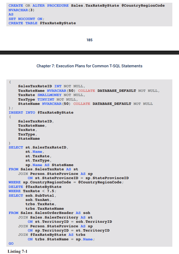
  1. CREATE TABLE #TaxRateByState – temp table for selected tax rates.

  2. INSERT rows from Sales.SalesTaxRate ☰ Person.StateProvince, filtered by @CountryRegionCode.

  3. DELETE rows in temp table where TaxRate < 7.5.

  4. SELECT final result set joining sales orders, territories, states and the temp table.

• Data-type note: parameter declared as NVARCHAR(3) because the underlying column is NVARCHAR(3); CHAR(3) would be more efficient but would trigger implicit conversions.

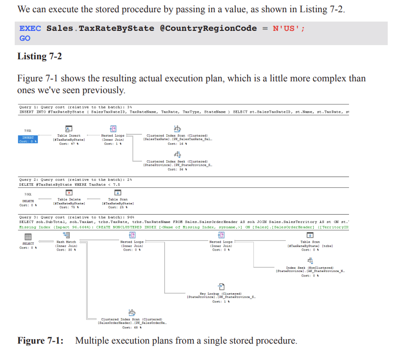
Execution-plan overview (Figure 7-1)

• Query 1: Populate temp table – $3\%$ of batch cost.

• Query 2: Delete low tax-rate rows – $1\%$ of batch cost.

• Query 3: Final SELECT – $96\%$ of batch cost and focus of tuning.

Parameter sniffing insight (Figure 7-2 / 7-3)

• Each compiled statement stores

  • Parameter Compiled Value – the value used during compilation (e.g. $N'US'$).

  • Parameter Runtime Value – the value used during the current execution.

• Steps at runtime:

  1. Batch is compiled; @CountryRegionCode for the outer EXEC is $N'US'$.

  2. Engine checks plan cache; if procedure plan missing it compiles and sniffs the parameter.

  3. Subsequent executions may reuse the plan even when runtime values differ.

  • Risk: if the compiled value’s selectivity is atypical, the reused plan may yield poor performance (see Chapter 8 on selectivity).

Detailed operators in Query 3 (Figure 7-4)

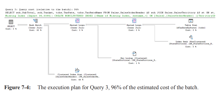
• Temp table scan (5 rows each executing separately) → outer input of Nested Loops.

• Inner input: Index Seek on StateProvince → returns matching state rows.

• Output feeds another Nested Loops; inner input: Key Lookup on StateProvince (fetching missing TerritoryID).

• Result becomes Build input to a Hash Match (join on TerritoryID).
  • Build side = 5 rows; Probe side = Clustered Index Seek on SalesOrderHeader (31 465 rows).
  • Hash table built in memory, matching returns 23 752 rows.

• Takeaway: procedure plans are regular execution plans; identify the costly section and apply the usual optimisation techniques (indexes, rewrites, statistics, etc.).

Subqueries

• A subquery is a SELECT embedded inside another SELECT/INSERT/UPDATE/DELETE.
  • Can appear in WHERE, SELECT, FROM, etc.
  • May be correlated (references outer query columns) or non-correlated.

• Pros: expressive, sometimes clearer than complex joins.

• Cons: may execute repeatedly (one execution per outer row) and prevent set-based optimisations.

Correlated subquery example (Listing 7-3)

SELECT p.Name, p.ProductNumber, ph.ListPrice
FROM Production.Product            AS p
INNER JOIN Production.ProductListPriceHistory AS ph
       ON p.ProductID = ph.ProductID
      AND ph.StartDate = (
             SELECT TOP (1) ph2.StartDate
             FROM Production.ProductListPriceHistory AS ph2
             WHERE ph2.ProductID = p.ProductID
             ORDER BY ph2.StartDate DESC);

• Objective: for each product return only the most recent price.

• Subquery is correlated through ph2.ProductID = p.ProductID.
  • Executes once per outer row to fetch latest StartDate.

Execution-plan outline (Figure 7-5)

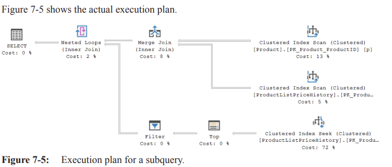
• Two Clustered Index Scans:
  • Production.Product (outer input).
  • Production.ProductListPriceHistory (inner input).

• Inputs feed a Merge Join on ProductID.
  • Ordered property for both scans = True (prerequisite for merge join).
  • The optimizer could not transform the query into a more efficient form (e.g. window functions, lateral joins) in this example, so full scans remain.

Performance considerations & alternatives

• Correlated subqueries on “versioned” history tables are common but may be sub-optimal.
  • Each product may require walking the entire history.

• Potential rewrites:

  • Use CROSS APPLY or OUTER APPLY with TOP (1) ... ORDER BY to allow index seeks.

  • Employ window functions: ROW_NUMBER() partitioned by ProductID ordered by StartDate DESC inside a CTE/derived table, then filter on ROW_NUMBER = 1.

  • Add/support indexes on (ProductID, StartDate DESC) to make the seek pattern efficient.

Real-world relevance & best practices

• Many production procedures grow organically; temporary tables, subqueries, and non-ideal datatypes are common.

• Knowing how SQL Server generates execution plans lets you
  • Diagnose hotspots quickly without rewriting entire modules.
  • Decide whether a small fix (index, hint) or a full rewrite (set-based logic, elimination of temp objects) yields the best ROI.

• Ethical/practical implication: touching legacy code requires balancing performance gains with stability and maintainability; sometimes “good enough” tuning is preferable to risky refactors.

Quick reference – numbers & statistics mentioned

• Temp table rows after delete: $5$

• SalesOrderHeader rows probed: $31\,465$

• Rows returned after hash join: $23\,752$

• Relative batch costs: Query 1 $3\%$, Query 2 $1\%$, Query 3 $96\%$

Ordered Retrieval & Merge Join Basics

• Two Clustered Index Scans are marked Ordered because of the clustered index on (ProductID) – the engine therefore uses the Ordered retrieval method.
• Merge Join exploits this ordering:
• Reads two ordered inputs simultaneously, locating matching rows on the join column.
• In the current example it emits $395$ joined rows (matching list-price rows).
• Atypical distribution noted: Products table contains $504$ rows, but only $395$ have list-price history – ideally every product would have ≥1 price entry.

Nested Loops Join – Row-by-Row Inner Execution

• Those $395$ Merge-Join rows feed the outer input of a Nested Loops (NL) join.
• Outer References: values from ProductID and StartDate are pushed to the inner input.
• Inner input = Clustered Index Seek on ProductListPriceHistory(ProductID, StartDate)
• A TOP (1)…ORDER BY StartDate DESC guarantees only the most-recent price per product.
• A Filter then accepts/rejects the single candidate row according to StartDate equality.
• Costly behaviour:
• Filter (and its child operators) executes $395$ times.
• NL only needs to know whether a row exists, so the Filter returns an empty row shell – no columns, just row-presence metadata.
• Startup Expression = False ➔ children execute on every outer row; had it been Startup Expression Predicate, children would run only when the predicate is met.
• Hypothetical illustration of the scan penalty:
• Suppose $200$ products × $15$ prices ⇒ $3000$ rows post-Merge-Join.
• NL would perform $3000$ inner seeks, each reading the same $200$ rows repeatedly ⇒ very high logical reads.

Tuning Idea 1 – Replace TOP(1)…ORDER BY with MAX()

• Query rewrite: SELECT MAX(ph2.StartDate)…
• Eliminates the TOP + NL pattern.
• Plan changes to two Merge Joins and shows lower I/O.

Derived Tables & APPLY – Fundamentals

• A derived table is a sub-query in the FROM clause, named with an alias; logically a “virtual table”.
• Before SQL Server 2005 all derived tables had to be independent; 2005 introduced APPLY to allow correlation:
• CROSS APPLY – like an inner join, discards rows when right side returns nothing.
• OUTER APPLY – like a left outer join, returns NULLs for missing right-side rows.
• Logical definition: right-side sub-query is evaluated once per left-side row (though the optimizer may implement differently).
• MSDN reference: http://bit.ly/1FFmldl

Tuning Idea 2 – CROSS APPLY Version (Listing 7-4)

SELECT p.Name,
       p.ProductNumber,
       ph.ListPrice
FROM   Production.Product p
       CROSS APPLY (
           SELECT TOP (1) ph2.ProductID,
                           ph2.ListPrice
           FROM   Production.ProductListPriceHistory ph2
           WHERE  ph2.ProductID = p.ProductID
           ORDER  BY ph2.StartDate DESC
       ) AS ph;

• Plan (Figure 7-9):

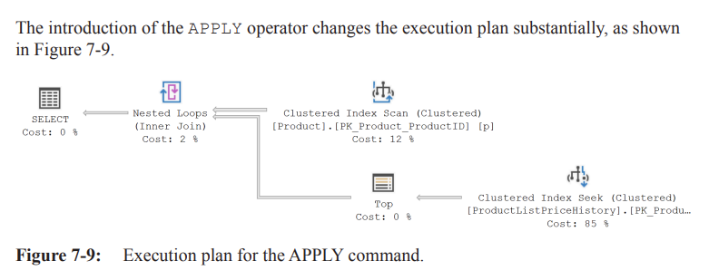
• Outer input: Clustered Index Scan on Products (produces $504$ rows).
• Inner input: Seek + TOP (1) on ProductListPriceHistory executed $504$ times.

Comparing I/O – Subquery (Listing 7-3) vs APPLY (Listing 7-4)

• Captured with Extended Events (Listing 2-6) – execution-plan capture disabled to avoid observer effect.
• Logical reads:
• Subquery in the JOIN: $811$ reads.
• CROSS APPLY version: $1024$ reads.
• Reason: NL inner executes $395$ times for the subquery vs $504$ times for APPLY.
• Note: This sample’s data distribution is unusual (many products lack prices). In a typical distribution (each product has many price rows) APPLY is expected to win.

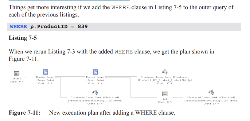
Subquery Plan Changes (Figure 7-11)

• Filter removed.
• TOP operator now appears on the outer (parent) branch instead of the subquery branch.
• Three Clustered Index Seeks + two Nested Loops:
• Right-most Seek (alias ph2) supplies the subquery’s most recent StartDate.
• Second Seek joins on both ProductID + StartDate pushed as Outer References.
• Each NL inner now executes once (outer input only 1 row) – huge I/O reduction.

APPLY Plan Changes (Figure 7-12)

• Plan identical, except outer Clustered Index Scan → Seek due to the predicate.

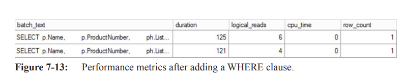
New I/O Metrics (Figure 7-13)

• APPLY query: $4$ logical reads.
• Subquery query: $6$ logical reads.
• APPLY consistently faster in repeated runs; advantage grows with larger data sets.

Key Take-aways on Plan Choice

• Always benchmark with representative data; small anomalies in distribution can sway the optimizer’s plan selection.
• Re-evaluate queries periodically as data grows or skews – plan & performance can change.
• Extended Events give low-overhead runtime metrics; avoid plan capture when measuring pure duration.

Common Table Expressions (CTEs) – Overview

• Introduced in SQL Server 2005.

• Behave like derived tables but

  • Exist only for the scope of a single statement.

  • Can be self-referential and reused multiple times in that statement.

  • Cannot be correlated (even with APPLY).

Recursive CTE Anatomy

• Composed of at least two queries combined with UNION ALL:

1. Anchor member – the base result set. (can be executed on its own to produce a result)

2. Recursive member – references the CTE itself, generating additional rows.
   • Logical execution: anchor ➔ feed rows to recursive member ➔ recursive member feeds itself until no more rows.

Example – dbo.uspGetEmployeeManagers

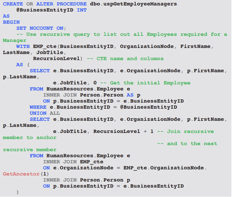
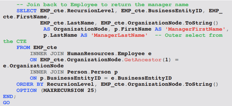
• Purpose: list a given employee and all managerial ancestors.

• Optimizer usually produces a Recursive Union operator followed by Nested Loops or Index Seeks for each iteration.

• Ex: EXEC dbo.uspGetEmployeeManagers @BusinessEntityID = 9

Practical / Ethical / Operational Implications

• Operational: High logical reads = buffer-pool pressure, longer execution time, risk of blocking; plan tuning mitigates these.
• Ethical: Running ill-performing queries on production systems wastes shared resources, potentially impacting SLAs and user experience.
• Practical: Choose query constructs (TOP vs MAX, subquery vs APPLY, CTE vs temp table) based on data size, distribution, and required use of intermediate results.

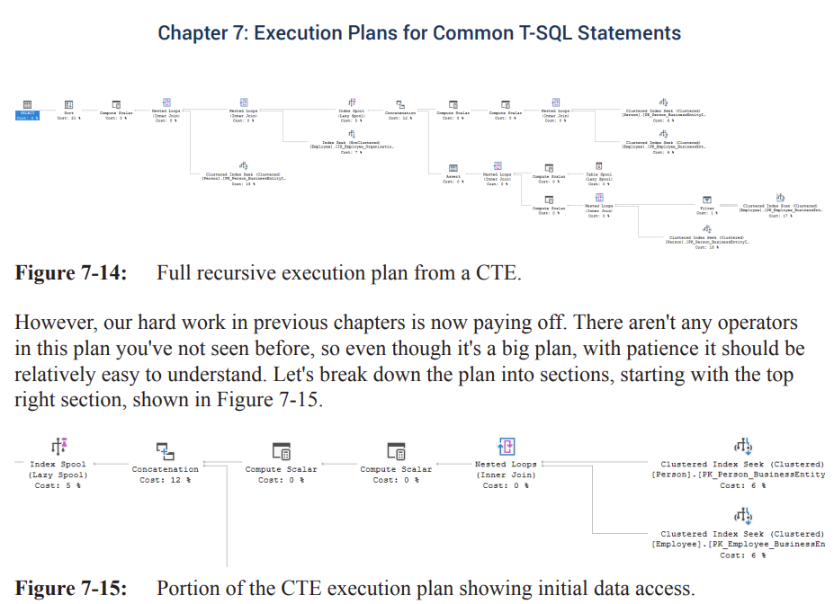
Operator Walk-Through (Logical Left-to-Right)

• Index Spool (Lazy) – NodeID $4$; first operator logically encountered.

  • Stores rows from Concatenation; acts as start of recursion.

  • Streams: requests 1 row from child, stores, immediately passes to parent.

• Concatenation – Implements $UNION\ ALL$.

  • Top input = Anchor member.

  • Bottom input = Recursive member.

  • Processes top until exhausted, then switches permanently to bottom.

Anchor Member Sub-Plan (Top Input)

• 2 Clustered Index Seeks

  • Tables: $HumanResources.Employee$ and $Person.Person$.

• Nested Loops join combines the two seeks.

• Returns 1 row (employee $ID = 9$).

• 2 Compute Scalar operators

  • Initialize $RecursionLevel = 0$ and derived column $RecursionLevel$.

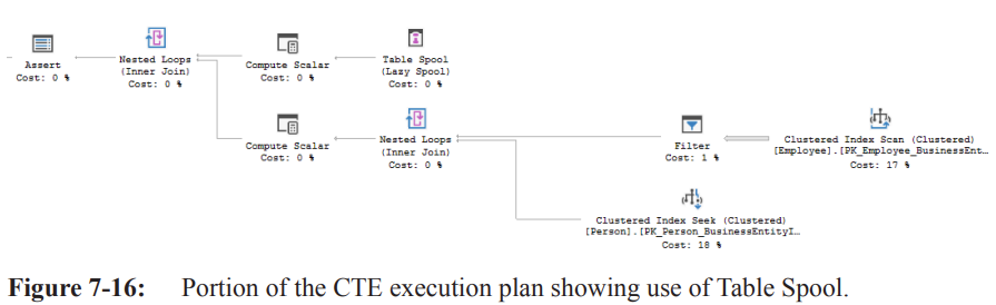
Recursive Member Sub-Plan (Bottom Input)

• Table Spool – NodeID $14$; Primary Node ID = $4$.

  • Property With Stack = True ⇒ behaves as stack (LIFO) – critical for recursion logic.

  • Reads a copy of each row stored by Index Spool, removes it after read.

• Assert

  • Enforces $MAXRECURSION\ (25)$; aborts execution if level exceeded.

• Compute Scalar next to Table Spool

  • Calculates new recursion level: $RecursionLevel = RecursionLevel + 1$.

• Outer input (from Table Spool) joins via Nested Loops to Employee and Person tables.

  • Join predicate uses $GetAncestor(1)$ on OrganizationNode.

• Clustered Index Scan – Employee

  • Estimated executions $4$; estimated rows/exec $290$ ⇒ $4 \times 290 = 1160$ rows.

  • Actual rows $= 1160$ (estimate matched).

• Filter

  • Performs comparison $OrganizationNode = GetAncestor(…)$ after full table scan.

  • Returns 1 manager row for first 3 iterations; returns 0 on CEO row ⇒ recursion ends.

Row Flow Summary

• Concatenation outputs $4$ rows (1 anchor + 3 recursive).

• Final extra join to grab manager names drops CEO row (no manager) ⇒ 3 rows returned to client.

Conceptual Insights & Best Practices

• Index Spool + Table Spool (stack) is SQL Server’s internal mechanism for recursive CTE evaluation.

• Assert operator is the physical manifestation of $MAXRECURSION$.

• Reading plans left-to-right (logical ordering) is essential for understanding recursion flow.

Views in Execution Plans

• A view = stored query; appears table-like but optimizer never “sees” it as a physical object.

  • During binding (Chapter 1), algebrizer expands the view into its base query.

• Developers often misuse views by joining view-to-view or nesting views ⇒ optimizer overwhelmed.

  • Recognized as a code smell; avoid!

Example – Standard View (Sales.vIndividualCustomer)

• Query 1 – SELECT * FROM Sales.vIndividualCustomer WHERE businessEntityId = 8743 (Listing 7-18)

  • Forces retrieval of every column; optimizer must access 8 tables / 7 joins defined in the view.

  • Plan in Figure 7-19: many operators, complex shape.

    

• Query 2 – Column list (Listing 7-9)

  • Requests only BusinessEntityID, Title, LastName, FirstName

  • Simplification phase removes unnecessary tables/columns.

  • Generates much smaller plan (Figure 7-21).

  • Simplification not perfect – e.g., EmailAddress table still present even though not strictly needed.

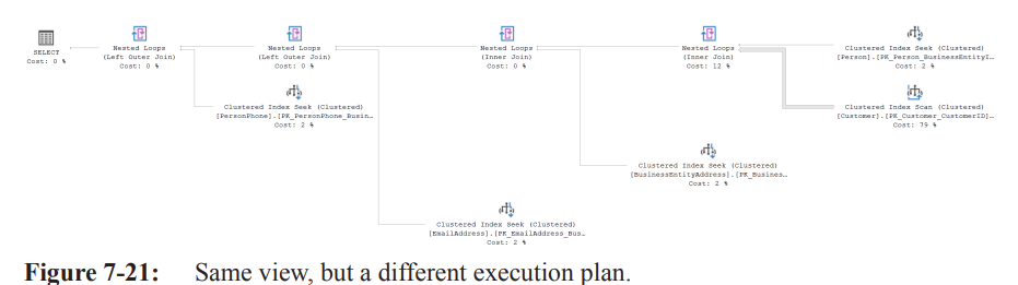
SELECT ic.BusinessEntityID,
 ic.Title,
 ic.LastName,
 ic.FirstName
FROM Sales.vIndividualCustomer AS ic
WHERE BusinessEntityID = 8743;

Key Takeaways for Standard Views

• Selecting fewer columns can dramatically change the plan due to simplification.

• Views improve developer productivity but do not reduce optimizer work; complexity is merely hidden.

Indexed (Materialized) Views

• Definition: View + Clustered Index ⇒ physically stores data like a table.

• Pros

  • Query performance boost: joins & lookups pre-computed, direct access via clustered index.

  • Particularly beneficial for aggregations & complex joins.

• Cons / Costs

  • Creation cost is high (one-time) – should be scheduled during low-load periods.

  • Maintenance overhead on DML (INSERT/UPDATE/DELETE) of base tables.

  • Example: If a base table receives $100$ inserts/min, each insert propagates into indexed view.

  • Evaluate trade-off: static base tables → low overhead; high-churn tables → potential performance hit.

Cross-Chapter Connections

• Spool behavior discussed in Chapter 5.

• Concatenation operator details covered in Chapter 4.

• Binding & algebrizer expansion of views explained in Chapter 1.

Practical & Ethical Implications

• Misusing views or over-nesting can mask inefficiencies, leading to production slowdowns – ethical obligation to write transparent, maintainable code.

• Indexed views must be designed with full understanding of workload to avoid unnecessary resource consumption.

Indexed Views: Rationale & Advantages

• Purpose of indexed views
  • Pre-aggregate or pre-join data once, at index-creation time, so subsequent queries can read pre-materialized results.
  • Eliminates repeated GROUP BY or aggregation logic on every execution.
  • Delivers substantial I/O savings because the data is already summarized.

• Key benefit sequence
  • Create view WITH “SCHEMABINDING”
  • This clause binds the view to the schema of the underlying base tables, preventing the base tables from being dropped or modified in a way that would affect the view definition. It's a mandatory requirement for creating clustered indexes on views.
  • Create unique clustered index
  • This step materializes the view, meaning the results of the view's query are stored physically on disk, similar to a regular table. A unique clustered index ensures data integrity and provides an efficient physical storage structure.
  • View becomes materialized
  • Once the unique clustered index is created, the data defined by the view is computed and stored. This materialization is the core power of indexed views, turning a logical view into a physical data structure.
  • Future SELECTs read only the index
  • When a query matches the definition of the indexed view, the SQL Server query optimizer can choose to read directly from the pre-computed clustered index instead of accessing and joining the underlying base tables, leading to significant performance gains.

Example: AdventureWorks2014 – vStateProvinceCountryRegion

• Complete DDL sequence (Listing 7-10)

DROP VIEW IF EXISTS Person.vStateProvinceCountryRegion;

CREATE OR ALTER VIEW Person.vStateProvinceCountryRegion
  WITH SCHEMABINDING
  AS
  SELECT sp.StateProvinceID, sp.StateProvinceCode, sp.IsOnlyStateProvinceFlag, sp.Name AS StateProvinceName,
         sp.TerritoryID, cr.CountryRegionCode, cr.Name AS CountryRegionName
  FROM Person.StateProvince AS sp
  INNER JOIN Person.CountryRegion AS cr ON sp.CountryRegionCode = cr.CountryRegionCode;

CREATE UNIQUE CLUSTERED INDEX IX_vStateProvinceCountryRegion
ON Person.vStateProvinceCountryRegion (StateProvinceID ASC, CountryRegionCode ASC);

– Columns: StateProvinceID, StateProvinceCode, IsOnlyStateProvinceFlag, StateProvinceName, TerritoryID, CountryRegionCode, CountryRegionName

• Execution-plan observations (Figure 7-22)
  • DDL generates a plan because SQL Server must execute the view-definition query to populate the clustered index.
  • Operators: Clustered Index Insert fed by Nested Loops join of the two base tables.

Querying an Indexed View

SELECT StateProvinceCode, IsOnlyStateProvinceFlag, CountryRegionName
FROM Person.vStateProvinceCountryRegion;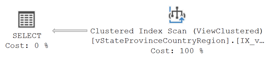

• In $Enterprise$ / $Developer$ Editions, optimizer matches directly to the indexed view.
• Resulting plan (Figure 7-23): single Clustered Index Scan on $IX_vStateProvinceCountryRegion$ (no join operators visible).
• In $Standard$ pre-2016 SP1 or $Express$, require $WITH\ (NOEXPAND)$ hint to force same behavior.

SELECT StateProvinceCode, IsOnlyStateProvinceFlag, CountryRegionName
FROM Person.vStateProvinceCountryRegion WITH (NOEXPAND);

Indexed-View Index Matching Outside the View

• Query (Listing 7-12) hits base tables, not the view

  SELECT sp.StateProvinceCode, sp.IsOnlyStateProvinceFlag, cr.Name AS CountryRegionName
  FROM Person.StateProvince AS sp
  INNER JOIN Person.CountryRegion AS cr ON sp.CountryRegionCode = cr.CountryRegionCode;

• Optimizer may still choose the indexed view’s index if it provides lowest cost.
• Plan still shows single Clustered Index Scan on the view’s clustered index (again edition-dependent).

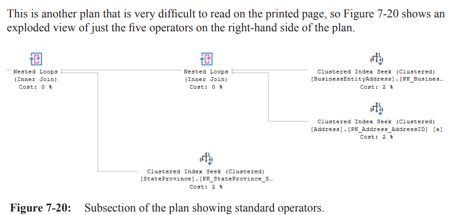
Limitations & Automatic Matching Failures

• As query complexity grows, automatic indexed-view matching may fail.
  • Example (Listing 7-13): join $Person.Address$ with the view and filter by $AddressID=22701$.

  SELECT pa.Color, spcr.StateProvinceName, spcr.CountryRegionName
  FROM Person.Address AS pa
  INNER JOIN Person.StateProvince AS sp ON pa.StateProvinceID = sp.StateProvinceID
  INNER JOIN Person.vStateProvinceCountryRegion AS spcr ON sp.StateProvinceID = spcr.StateProvinceID
  WHERE pa.AddressID = 22701;

• Plan (Figure 7-24) shows “view expansion”: optimizer substitutes base tables from view definition, then performs join.

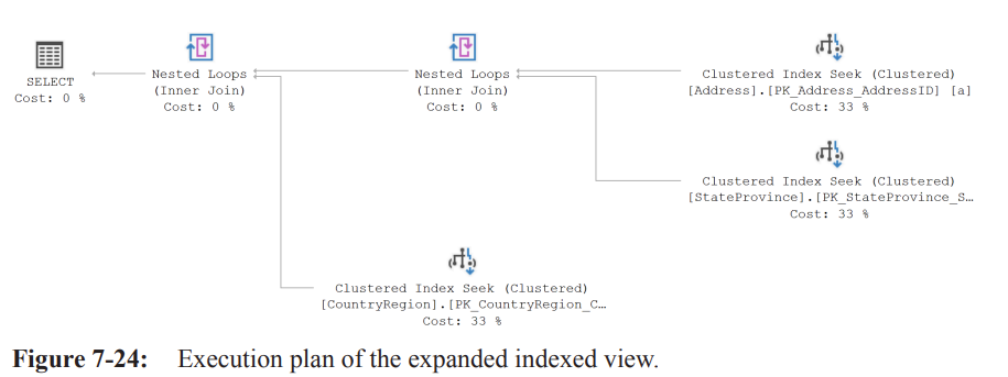
• Reasons
  • Algebrizer always expands views.
  • Optimizer estimates direct table access cheaper than using materialized index.

• Work-around
  • Use $NOEXPAND$ hint to force use of indexed view (detailed in Chapter 10).

  SELECT pa.Color, spcr.StateProvinceName, spcr.CountryRegionName
  FROM Person.Address AS pa
  INNER JOIN Person.StateProvince AS sp ON pa.StateProvinceID = sp.StateProvinceID
  INNER JOIN Person.vStateProvinceCountryRegion WITH (NOEXPAND) AS spcr ON sp.StateProvinceID = spcr.StateProvinceID
  WHERE pa.AddressID = 22701;

Functions Overview

• Two user-defined function (UDF) categories
  • Scalar UDFs – return single value.
  • Table-valued UDFs – return table expression.

• Execution-plan handling can be deceptive; much work hidden behind a Compute Scalar.

Scalar UDF Example – dbo.ufnGetStock

• Definition (Listing 7-14)

  CREATE FUNCTION dbo.ufnGetStock (@ProductID INT)
  RETURNS INT
  AS
  BEGIN
      DECLARE @ret INT;
      SELECT @ret = SUM(Quantity)
      FROM Production.ProductInventory
      WHERE ProductID = @ProductID AND LocationID = '6';

      IF @ret IS NULL
          SET @ret = 0;

      RETURN @ret;
  END;

• Parameters: $@ProductID\ int$
• Logic
– $SELECT\ @ret=SUM(Quantity)\ FROM\ Production.ProductInventory\ WHERE\ ProductID=@ProductID\ AND\ LocationID='6';$
– If $@ret$ $IS\ NULL$ then set $@ret=0$.
– $RETURN\ @ret;$

• Caller query (Listing 7-15)

  SELECT p.Name, dbo.ufnGetStock(p.ProductID) AS StockLevel
  FROM Production.Product AS p
  WHERE p.Color = 'Black';

• $SELECT\ p.Name,\ dbo.ufnGetStock(p.ProductID)\ AS\ StockLevel\ FROM\ Production.Product\ p\ WHERE\ p.Color='Black';$
• Returns $93$ rows.

Actual-plan View (Figure 7-25)

• Operators
  • Clustered Index Scan on $Production.Product$ ➔ Predicate $Color='Black'$.
  • Compute Scalar calls scalar UDF once per row (hidden).

• Why only two operators?
  • Actual plan in SSMS collapses scalar-UDF details; you must inspect Defined Values within Compute Scalar to see the function invocation.

Estimated-plan View (Figure 7-27)

• Reveals two separate plans
  • Main query plan (as above).
  • Nested plan for the scalar UDF.

• Scalar UDF internal plan breakdown (Figure 7-30 reference)
  • Root operator: $UDF$ (T-SQL operator) with overall estimated cost.
  • Sub-branch 1 – SELECT
  – Clustered Index Seek on $Production.ProductInventory$ filtering by $ProductID$ and $LocationID=6$.
  – Stream Aggregate to $SUM(Quantity)$.
  – Compute Scalar to assign $@ret$.
  • Sub-branch 2 – $COND$ (NULL check)
  – If $@ret\ IS\ NULL$ ➔ $ASSIGN$ sets $@ret=0$.
  • Sub-branch 3 – $RETURN$ operator outputs $@ret$.

Performance Implications of Scalar UDFs

• Hidden cost
  • UDF executes once per outer row ➔ $93$ executions in example.
  • Each execution repeats the internal plan (Seek ➔ Aggregate ➔ etc.).

• Misleading STATISTICS IO
  • Reported logical reads for main query: $15$.
  • Actual cumulative reads when including UDF executions: $211$.
  • Rows touched: $365$ total across all UDF calls vs. $93$ reported.

• Takeaway
  • Inline the logic (e.g., join to $ProductInventory$ directly) to avoid repetitive execution and reduce I/O.

  SELECT p.Name, ISNULL(SUM(inv.Quantity), 0) AS StockLevel
  FROM Production.Product AS p
  LEFT JOIN Production.ProductInventory AS inv
      ON p.ProductID = inv.ProductID AND inv.LocationID = '6'
  WHERE p.Color = 'Black'
  GROUP BY p.Name;

Key Takeaways & Best Practices

• Indexed views
  • Great for pre-computed aggregations or joins; ensure appropriate edition or use $NOEXPAND$.
  • Always evaluate whether optimizer automatically chooses the index; inspect plans.

• Scalar UDFs
  • Can hide significant work; prefer inline TVFs or rewrite as joins/expressions when performance matters.
  • Use estimated plans or Extended Events to expose hidden cost and validate true I/O.

• General
  • Always analyze both actual and estimated plans for DDL, views, and UDFs to uncover non-obvious operators and costs.
  • Remember that STATISTICS IO/Time on the outer query may omit nested UDF activity; use XEvents or DMVs for full picture.

Overview of Table-Valued Functions (TVFs)

• Two distinct varieties, each with different behavioral & optimization characteristics:

  • Inline Table-Valued Functions (iTVFs)
    • Also called parameterized views because they behave like a view whose definition can accept parameters.
    • Contain exactly one SELECT statement returned by the RETURN() clause.
    • No body (BEGIN…END) and no intermediate table variable.

  • Multi-Statement Table-Valued Functions (mTVFs)
    • Contain a declared table variable returned to the caller.
    • Allow multiple INSERT, UPDATE, DELETE, control-flow, etc.
    • Behave similarly to scalar UDFs with respect to plan opacity and cardinality estimation.

• Both expose a table result, but appear very differently in execution plans.

Inline TVF (iTVF)

• Example rewritten from Listing 7-14 (Listing 7-16):

  CREATE FUNCTION dbo.GetStock (@ProductID INT)
  RETURNS TABLE
  AS
  RETURN (
      SELECT SUM(pi.Quantity) AS QuantitySum
      FROM Production.ProductInventory AS pi
      WHERE pi.ProductID = @ProductID
        AND pi.LocationID = '6'
  );

• Query that consumes the function (Listing 7-17):

  SELECT p.Name, gs.QuantitySum
  FROM Production.Product AS p
  CROSS APPLY dbo.GetStock(p.ProductID) AS gs
  WHERE p.Color = 'Black';

• Key attributes:

  • Appears to optimizer as a single expanded query; no hidden operators.

  • Allows all cost estimates & statistics to flow naturally.

  • Can participate in parallel plans, inlining, predicate push-down, etc.

Execution Plan for iTVF (Figure 7-28)

• No aggregation operator present even though the SELECT contains SUM(pi.Quantity):

  • Optimizer notices that predicate LocationID = 6 combined with a unique index on (ProductID, LocationID) guarantees ≤ 1 row / product.

  • Therefore $\text{SUM}(Quantity)$ is the same as the raw Quantity value → aggregation eliminated.

• Left-to-right operator flow:

  • Merge Join (Right Outer) between ProductInventory & Product.

  • Clustered Index Scan (ProductInventory) with predicate push-down on LocationID = 6.

  • Compute Scalar converts SMALLINT Quantity → INT because aggregation would normally promote the type; with no explicit aggregate the conversion is done here.

  • Clustered Index Scan (Product) provides product rows filtered later by p.Color = 'Black'.

• Plan characteristics:

  • Estimated & Actual plans are identical except for runtime row counts.

  • Full cost visibility; cardinality is accurate.

Multi-Statement TVF (mTVF)

• Rewritten example (Listing 7-18):

  CREATE FUNCTION dbo.GetStock2 (@ProductID INT)
  RETURNS @GetStock TABLE (QuantitySum INT NULL)
  AS
  BEGIN
      INSERT @GetStock (QuantitySum)
      SELECT SUM(pi.Quantity)
      FROM Production.ProductInventory AS pi
      WHERE pi.ProductID = @ProductID
        AND pi.LocationID = '6';
      RETURN;
  END

• Consuming query identical to Listing 7-17 except call dbo.GetStock2.

• Fundamental differences:

  • Internally uses a table variable (@GetStock).

  • Generates its own sub-plan that is hidden behind a single Table Valued Function operator in the outer plan.

  • Disallows cost-based rewrites, parallelism, & predicate push-down for the body.

Execution Plan for mTVF (Figure 7-29)

• Outer plan now shows:

  • Nested Loops join where the inner side is a single Table Valued Function operator.

  • Other operators (e.g., scan on Product) remain visible.

• Properties of the Table Valued Function operator (Figure 7-30):

  • Estimated Number of Rows = $100$ (hard-coded default for table variables in SQL Server 2014+; pre-2014 it was $1$).

  • Estimated number of executions = $93$ (one per outer row).

  • Total estimated rows $= 100 \times 93 = 9300$ vs. actual $= 1 \times 93 = 93$.

  • Large mismatch drives sub-optimal join choice & memory grants.

• Hidden inner plan (Figure 7-31):

  • Resembles scalar UDF pattern:
    • Table Insert → inserts into table variable.
    • Clustered Index Scan on ProductInventory.
    • Hash/Aggregate or Compute Scalar etc.

  • This work is executed once per outer row → significant cumulative cost.

Cardinality Estimation & Hard-Coded Defaults

• For any table variable (used by mTVF), cardinality estimator lacks statistics → uses fixed default.

  • $\text{Pre-2014 default} = 1$ row.

  • $\text{SQL Server 2014+ default} = 100$ rows.

• Because the default is divorced from reality, join ordering and memory grants can be severely skewed.

Performance Implications & Hidden Costs

• iTVF:
  • Fully exposes logic; optimizer can eliminate aggregates, push predicates, choose efficient joins.
  • No hidden batch iterations.

• mTVF:
  • Appears as black-box to outer query; internal cost not considered.
  • Executed row-by-row if placed on inner side of loops join → "triangular" execution pattern (N outer × M inner).
  • Example I/O jump: iTVF = $44$ reads vs. mTVF = $1141$ reads (≈ 26× increase).

• Similarity to scalar UDFs:
  • Both hide computations; both default to row-by-row execution; both hinder parallelism.

Comparison Summary

• Scalar UDF
  • Returns single value; hidden internal plan; executes per row.

• Inline TVF
  • Returns tabular result; inlined into outer query; full cost visibility.

• Multi-Statement TVF
  • Returns tabular result via table variable; hidden plan; suffers from default cardinality $=100$.

Practical Guidelines / Best Practices

• Prefer inline TVFs whenever possible for reusable, parameterized table logic.

• Avoid multi-statement TVFs unless absolutely necessary; consider:
  • Rewriting as inline TVF or view + parameters.
  • Converting to stored procedure with OPTION (RECOMPILE) if row-by-row semantics unavoidable.

• If you must use mTVF:
  • Capture execution stats & monitor for row mis-estimation.
  • Use OPTION (USE HINT('DISABLE_TFP')) in newer versions to force scalar/multi-statement function inlining if supported.
  • In SQL Server 2019+, enable Scalar UDF/Multi-Statement TVF Inlining feature for automatic plan expansion.

• Always inspect:
  • Estimated vs. Actual rows on the Table Valued Function operator.
  • Nested Loops inner vs. Hash/Batch modes to catch row-by-row hotspots.

Key Takeaways

• Execution-plan visibility dictates optimizer effectiveness.
  • iTVF → transparent; mTVF/scalar UDF → opaque.

• Hard-coded cardinality defaults (1 or 100) can mislead the optimizer, causing excessive I/O & CPU.

• Reading complex plans follows the same core principles:
  • Start at leftmost/rightmost iterator (depending on display order).
  • Check properties, row flow, join types.

• Larger plans are not fundamentally different—just require more systematic operator-by-operator analysis.