Chapter 3 Microeconomics: Supply and Demand

Markets

A market is any institutional arrangement that allows buyers and sellers to interact and thereby determine price and quantity. In practical terms the term stretches from a face-to-face farmer’s stall in a village square to the electronic trading pit of the New York Stock Exchange. Three geographical scales are normally distinguished. A strictly local market—say, the Saturday farmers’ bazaar—limits itself to neighbourhood participants. A national market, such as the U.S. real-estate market, unites dispersed agents within one political jurisdiction. Finally, an international market, e.g. global equity trading centred on Wall Street, links buyers and sellers across borders. In every one of these arenas the money price that ultimately prevails is the spontaneous outcome of countless bids made by consumers and asks posted by producers. Whenever we speak of “price discovery” we are referring to this decentralized and continuous haggling that pushes the market toward a single transactional price.

Demand

Economists use the noun “demand” to denote an entire schedule or curve, never a single number. The idea is to record the various quantities a consumer (or an entire market of consumers) is both willing and able to purchase at each alternative price, holding all non-price influences constant (the ceteris paribus clause). An individual demand curve therefore reflects one person’s preferences and constraints, whereas a market demand curve horizontally sums the quantities demanded by all individuals at each price point.

The Law of Demand

The most stable empirical regularity in microeconomics is the inverse relation between price and quantity demanded: as the price falls quantity demanded rises, and vice-versa, all else equal. Formally we can write dPdQd​<0 or Qd=f(P)Qd=f(P) with a negative slope. Three mutually reinforcing explanations underpin this law:

1. The substitution effect: when the price of a good drops, it becomes relatively cheaper than its substitutes, prompting consumers to re-allocate expenditure toward it.

2. The income effect: a lower price effectively increases real income, allowing consumers to buy more of all normal goods, the good in question included.

3. Diminishing marginal utility: successive units of a good yield progressively less additional satisfaction, so only a lower price can coax buyers to absorb larger quantities.

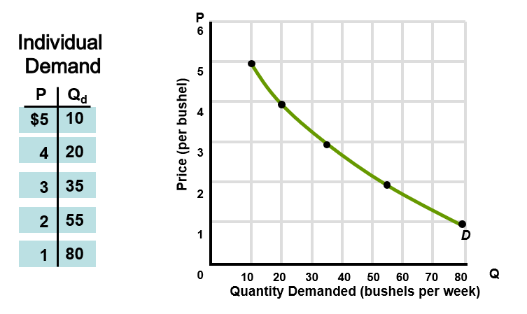
A Numerical Example—Individual Demand for Corn

Consider the following price–quantity pairs for a single buyer of corn (weekly purchases): {(P,Q_d)}={(\$5,10),(\$4,20),(\$3,35),(\$2,55),(\$1,80)}. Plotting these points and joining them with a smooth downward line gives the familiar negatively-sloped demand curve.

Market Demand

Suppose three consumers—Joe, Jen, and Jay—operate in the corn market. At P=\$3 Joe wants 35 bushels, Jen 39, and Jay 26. Horizontal addition furnishes the market total Q_d^{\text{market}}=100 bushels. Repeating the process for each price row yields the complete market demand schedule.

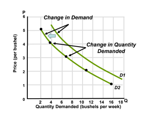
Movements Along vs. Shifts of the Demand Curve

A change in quantity demanded refers to a movement from one point to another along the same curve and is provoked solely by a price change. By contrast, a change in demand means the entire curve moves rightward (increase) or leftward (decrease) because some non-price determinant has altered. Graphically the distinction is captured by two separate curves, say D1 and D2, displaced in the horizontal dimension.

Determinants That Shift Demand

1. Tastes and preferences: a social craze for fitness, for example, swells demand for running shoes while shrinking demand for sedentary entertainment devices.

2. Number of buyers: a fall in the birth rate contracts demand for toys.

3. Income: higher household earnings lift demand for normal goods (restaurant meals, diamond necklaces) but depress demand for inferior goods (cheap wine, cabbage).

4. Prices of related goods: a fall in airfare (a substitute for rail travel) decreases rail demand; a drop in DVD-player prices (a complement) boosts DVD-movie demand.

5. Consumer expectations: news of an inclement coffee harvest in Brazil can induce today’s buyers to stockpile beans before the future price spike.

Each determinant operates by shifting the entire demand schedule to new positions D3, D4, etc. in diagrams.

Supply

Supply, like demand, is a complete schedule indicating the quantities a seller (or group of sellers) is willing and able to off-load at various prices, holding other influences constant. Individual supply deals with one firm, whereas market supply sums across many firms.

The Law of Supply

All else equal, quantity supplied varies directly with price. Algebraically dPdQs​>0 or Qs=g(P)Qs=g(P) with a positive slope. The logic is straightforward: a higher output price promises greater profit, providing an incentive to expand production. Nonetheless, as output rises the producer typically encounters rising marginal cost because of diminishing marginal returns, so increasingly higher prices are needed to elicit larger quantities.

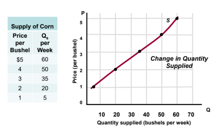
A Numerical Example—Supply of Corn

A hypothetical farmer’s weekly supply schedule might read {(P,Q_s)}={(\$1,5),(\$2,20),(\$3,35),(\$4,50),(\$5,60)}. Connecting the points yields an upward-sloping supply curve.

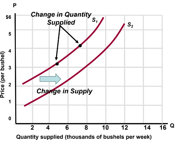
Movements Along vs. Shifts of the Supply Curve

A change in quantity supplied is the direct price-induced slide along a given curve. A change in supply denotes an autonomous shift of the curve—either rightward (increase) or leftward (decrease)—because of non-price factors. Graphs featuring multiple supply curves S1, S2, S_3 visualize the difference.

Determinants That Shift Supply

1. Resource prices: cheaper microchips expand computer supply; dearer crude oil throttles gasoline supply.

2. Technology: wireless breakthroughs augment the supply of mobile phones.

3. Taxes and subsidies: a higher cigarette excise shrinks cigarette supply, whereas a university subsidy cut reduces higher-education slots.

4. Prices of other goods: if pineapples command higher prices, farmers may reallocate acreage away from watermelons, decreasing watermelon supply.

5. Producer expectations: anticipation of future log price hikes induces present curtailment of timber harvesting.

6. Number of sellers: an influx of pharmacists enlarges the market supply of pharmaceutical services.

Market Equilibrium

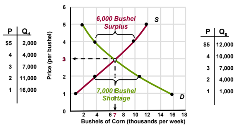
Equilibrium emerges at the price P^ and quantity Q^ where the plans of buyers and sellers mesh, mathematically the intersection point satisfying Qd(P)=Qs(P)Qd(P)=Qs(P). In the corn example the curves cross at P=$3P=$3 and Q=7,000Q=7,000 bushels per week.

When price strays above equilibrium a surplus materializes—here Qs>Qd, e.g. 12,000−7,000=5,00012,000−7,000=5,000 extra bushels at P=$5P=$5. Competitive sellers respond by bidding price down. Conversely, at P=$1 P=$1 the market suffers a shortage of 7{,}000 bushels (demand exceeds supply) and frustrated buyers bid price upward. This automatic adjustment is christened the rationing function of prices: the free-moving price is the most efficient instrument for eliminating excesses on either side and steering the market back to P^*.

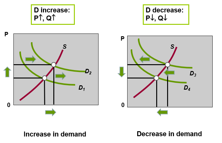
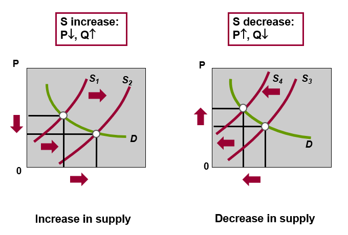
Comparative Statics—Demand or Supply Shifts

Suppose only demand shifts. A rightward shift (increase) lifts both equilibrium price and quantity: \Delta D>0 \Rightarrow P\uparrow ,\, Q\uparrow. A leftward shift does the opposite. If instead only supply shifts, a rightward shift lowers price but raises quantity (since products become more abundant), whereas a leftward shift raises price and shrinks quantity.

Simultaneous Shifts (Complex Cases)

The table of four archetypal scenarios summarises the ambiguous or determinate outcomes:

1. Supply increases while demand decreases ⇒ equilibrium price falls, equilibrium quantity indeterminate.

2. Supply decreases while demand increases ⇒ equilibrium price rises, equilibrium quantity indeterminate.

3. Both increase ⇒ quantity definitely rises, price indeterminate.

4. Both decrease ⇒ quantity definitely falls, price indeterminate.

Ambiguity arises because the curves move in two dimensions; without numeric magnitude we cannot foresee which effect dominates.

Government-Set Prices

In the name of equity or political expediency authorities sometimes override market outcomes. Two textbook interventions are:

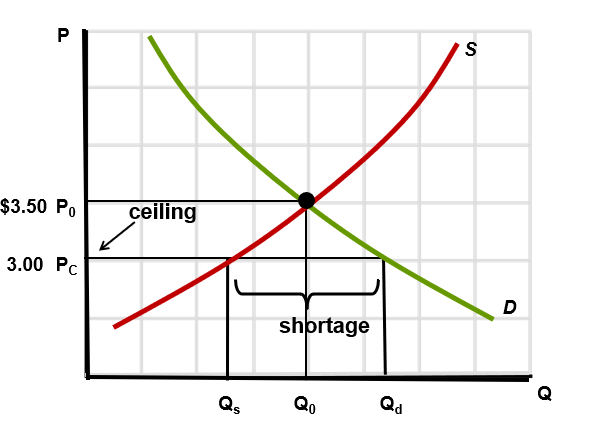
 Price Ceilings

A ceiling sets a legal maximum price Pc below P^. Because Pc, quantity demanded exceeds quantity supplied, producing a chronic shortage. Concert tickets, rent controls, and wartime ration books are historical illustrations. Secondary markets often emerge (black markets) where the good trades at an illegally high price. Socially, queuing, favouritism, and bribes may reallocate the scarce supply, undermining the intended fairness.

Graphically, if P^*=\$3.50 and legislators cap the price at Pc=\$3.00, the horizontal distance between Qd and Qs at Pc measures the shortage.

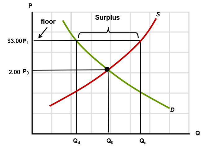
Price Floors

A floor imposes a legal minimum price Pf above P^. Typical examples include minimum-wage statutes and agricultural support programmes. Because Pf>P^, quantity supplied exceeds quantity demanded, yielding a surplus (unemployment in the labour market). Governments often purchase or store the excess, tax away the cost, or let surplus goods spoil—each option bearing economic and ethical costs.

In the illustration a floor at Pf=\$3.00 raises the legal price above the market level of \$2.00, leaving suppliers with unsold stock equal to Qs-Q_d.

Broader Significance & Ethical Overtones

Demand and supply analysis equips policymakers and business strategists to predict the direction (though not always the magnitude) of price and volume adjustments. Ethically, the notion that freely moving prices allocate resources “efficiently” collides with social goals such as affordability, wage security, and regional balance. While ceilings may protect low-income renters from exorbitant housing costs, they also discourage landlords from maintaining properties. Likewise, supporters champion minimum wages as a means of living-standard enhancement, yet opponents point to possible job losses among the least skilled. A recurrent theme is therefore the trade-off between equity (fairness) and efficiency (maximising the pie).

Finally, the law of diminishing marginal utility and the law of diminishing marginal product serve as conceptual foundations for much of consumer theory and production theory encountered in later chapters. Understanding them here clarifies why both demand and supply slopes look the way they do, and why equilibrium remains such a powerful predictive idea across real-world markets.