Study Notes: Exponential Growth and Decay in AP Calculus AB

The Proportionality Relationship

In AP Calculus AB, Exponential Models arise specifically from differential equations where the rate of change of a quantity is directly proportional to the current amount of that quantity. This is a fundamental application of Unit 7: Differential Equations.

When you read a problem statement that says:

"The rate of change of $y$ with respect to time $t$ is proportional to $y$."

You must immediately interpret this as the differential equation:

$\frac{dy}{dt} = ky$

Key Variables

• $y(t)$: The quantity at time $t$ (e.g., population, mass of an isotope).
• $t$: Time.
• $k$: The constant of proportionality.
• $\frac{dy}{dt}$: The instantaneous rate of change.

Deriving the General Model

While the final formula is often memorized, the AP exam requires you to know how to derive it using separation of variables. This proves that only the exponential function has a derivative proportional to itself.

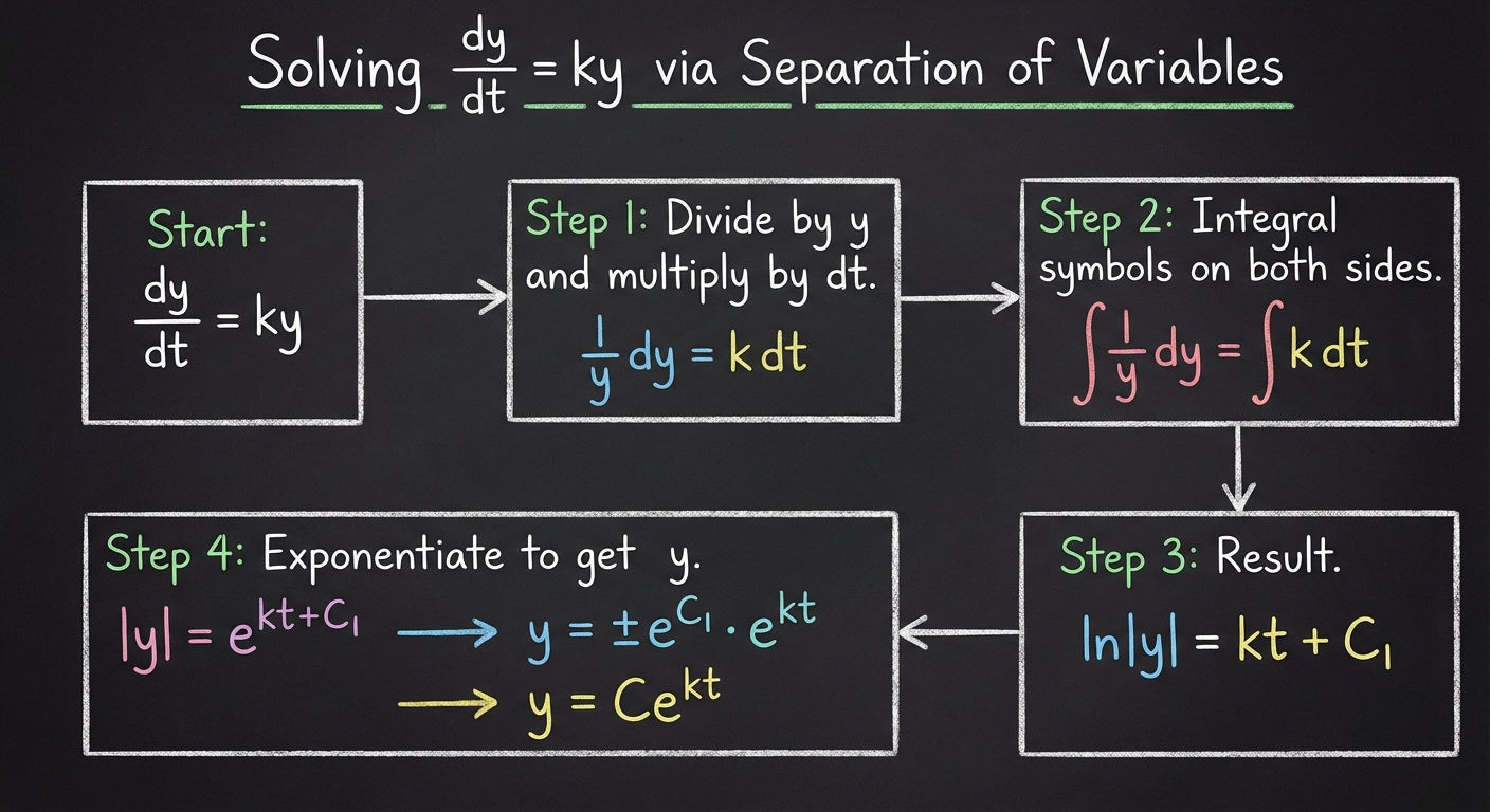
1. Separate Variables:
   Move all terms with $y$ to the left and $t$ to the right.
   $\frac{1}{y} \, dy = k \, dt$

2. Integrate Both Sides:
   $\int \frac{1}{y} \, dy = \int k \, dt$
   $\ln|y| = kt + C_1$

3. Exponentiate:
   To isolate $y$, make both sides powers of $e$.
   $|y| = e^{kt + C<em>1}$$|y| = e^{kt} \cdot e^{C</em>1}$

4. Define the Constant:
   Let $C = \pm e^{C_1}$. Since $y$ usually represents a physical quantity like population (which is positive), we can drop the absolute value and write:
   $y = Ce^{kt}$

The Result: The Law of Exponential Change

The general solution to $\frac{dy}{dt} = ky$ is always:

$y(t) = y_0 e^{kt}$

where:

• $y_0$ (or $C$) is the initial value at time $t=0$.
• $k$ is the growth constant ($k > 0$) or decay constant ($k < 0$).

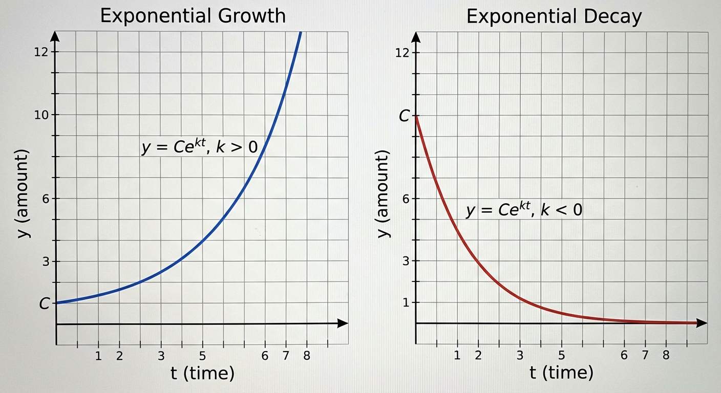
Growth vs. Decay

The behavior of the model depends entirely on the sign of $k$.

Exponential Growth ($k > 0$)

Occurs when the rate of increase is proportional to the current size. As $t \to \infty$, $y \to \infty$.

• Applications: Unrestrained population growth, compound interest, spread of a virus in early stages.
• Equation: $\frac{dy}{dt} = ky$ where $k$ is positive.

Exponential Decay ($k < 0$)

Occurs when the rate of decrease is proportional to the current size. As $t \to \infty$, $y \to 0$.

• Applications: Radioactive half-life, drug elimination from the bloodstream.
• Equation: $\frac{dy}{dt} = ky$ where $k$ is negative (often written as $\frac{dy}{dt} = -ky$ for clarity, where $k>0$, resulting in $y = y_0 e^{-kt}$).

Worked Examples

Example 1: Bacterial Growth

Problem: The number of bacteria in a culture is increasing at a rate proportional to the number of bacteria present. At time $t=0$ hours, there are 200 bacteria. At $t=2$ hours, there are 600 bacteria. Find an expression for the number of bacteria $y(t)$ at any time $t$.

Solution:

1. Identify the Model: Since the rate is proportional to the amount, $y = Ce^{kt}$.
2. Use Initial Condition: At $t=0, y=200$.
   $200 = Ce^{k(0)} \implies C = 200$
   So, $y = 200e^{kt}$.
3. Find $k$: Use the second point $(2, 600)$.
   $600 = 200e^{k(2)}$
   $3 = e^{2k}$
   Take $\ln$ of both sides:
   $\ln(3) = 2k \implies k = \frac{\ln(3)}{2} \approx 0.549$
4. Final Equation:
   $y(t) = 200 e^{\left(\frac{\ln 3}{2}\right)t}$

Example 2: Radioactive Decay (Half-Life)

Problem: A radioactive isotope decays at a rate proportional to its mass. The half-life of the isotope is 10 years. If the initial mass is 50 grams, when will only 5 grams remain?

Solution:

1. Understand Half-Life: Half-life is the time it takes for $y$ to become $\frac{1}{2}y<em>0$. This relationship allows us to find $k$ without knowing the specific mass amounts. $\frac{1}{2}y</em>0 = y_0 e^{k(10)}$
   $0.5 = e^{10k}$
   $k = \frac{\ln(0.5)}{10} = \frac{-\ln(2)}{10} \approx -0.0693$
2. Set up the specific equation: With $y_0 = 50$, the equation is:
   $y(t) = 50e^{-0.0693t}$
3. Solve for Time: Set $y(t) = 5$.
   $5 = 50e^{-0.0693t}$
   $0.1 = e^{-0.0693t}$
   $\ln(0.1) = -0.0693t$
   $t = \frac{\ln(0.1)}{-0.0693} \approx 33.22 \text{ years}$

Common Mistakes & Pitfalls

1. Neglecting the Initial Value ($C$)

   • Mistake: Assuming $y = e^{kt}$.
   • Correction: Always include the integration constant $C$ (which becomes the initial value $y_0$). The function tells you the ratio of growth, but the scale depends on where you started.

2. Confusion over Rate Language

   • Mistake: Applying the exponential model to a problem stating "rate of change is proportional to time."
   • Correction: Read carefully.
     • Proportional to $y$: $\frac{dy}{dt} = ky$ (Exponential).
     • Proportional to $t$: $\frac{dy}{dt} = kt$ (Quadratic, $y = \frac{1}{2}kt^2 + C$).

3. Algebraic Errors with Natural Logs

   • Mistake: Solving $3e^{kt} = 10$ by writing $\ln(3e^{kt}) = \ln(10)$ and incorrectly simplifying the left side.
   • Correction: Isolate the exponential term before taking the natural log. Divide by 3 first: $e^{kt} = \frac{10}{3}$, then $\ln$.

4. Sign Errors with Decay

   • Mistake: Calculating a positive $k$ for a decay problem and getting a function that grows.
   • Correction: Sanity check your answers. If the problem is about half-life or decay, your $k$ must be negative (or entered as a negative exponent).