Chapter 7 - Estimating Parameters(1)

Chapter 7 - Estimating Parameters

Point Estimate: A single value used to estimate a population parameter. This is directly taken from a particular sample.
Interval Estimate: A range of values that aims to estimate the true value of a population parameter, typically referred to as confidence intervals.

Definition: Each confidence interval has a corresponding confidence level, which represents the proportion of the sampling distribution it encompasses.
Higher confidence levels lead to wider intervals, while larger sample sizes typically result in narrower intervals.

Scenario: An inspector checks 60 washers, finding 12 damaged. Calculate a 95% confidence interval for the proportion of damaged appliances during shipment.

Example: To estimate if 25% of adults over 50 never graduated high school, determine how many individuals aged 25-30 must be surveyed to achieve a ±6% margin with 90% confidence.
Another example involves estimating the proportion of students using university shuttle services with ±3% accuracy using a 99% confidence level.

The t-distribution is utilized when the population standard deviation is unknown and especially useful for smaller sample sizes.
As the sample size increases, the t-distribution approaches a normal distribution.

Used when the population standard deviation is unknown. It is influenced by the degrees of freedom (n-1), where n is the sample size.
The shape of the t-distribution is typically wider than that of a normal distribution.

Random Sample: Ensures that the data is collected randomly.
Sampling Distribution Approximation: For n > 30, the distribution can be considered approximately normal.

A hospital samples 100 patients with a mean stay of 4.53 days and a standard deviation of 3.68. Calculate a 95% confidence interval for the mean length of stay.
### Example Problem: Hospital Stay - **Scenario**: A hospital samples 100 patients with a mean stay of 4.53 days and a standard deviation of 3.68. - **Objective**: Calculate a 95% confidence interval for the mean length of stay. - **Steps to Calculate**: 1. **Sample Size (n)**: 100 2. **Standard Error (SE)**: \[ SE = \frac{s}{\sqrt{n}} = \frac{3.68}{10} = 0.368 \] 3. **Critical Value for 95% Confidence Level**: t = 1.984 (df = 99). 4. **Margin of Error (ME)**: \[ ME = t \times SE = 1.984 \times 0.368 \approx 0.730 \] 5. **Confidence Interval**: - **Lower Limit**: 4.53 - 0.730 \approx 3.80 - **Upper Limit**: 4.53 + 0.730 \approx 5.26 - **Result**: 95% Confidence Interval for the mean length of stay: (3.80 days, 5.26 days).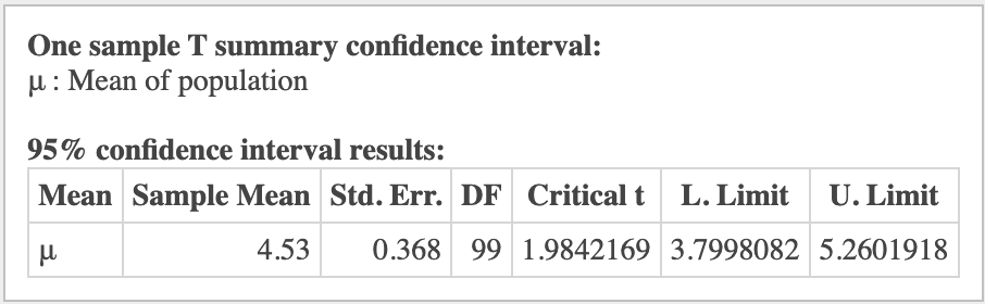
Suppose an archeologist randomly discovers 6 fossil skeletons from a previously unknown species of miniature horse. Reconstruction of the skeletons allows her to measure their shoulder height (in centimeters) of the horses. The heights are 45.3, 47.1, 44.2, 46.8, 45.5, and 47.6. From this data construct a 95% confidence interval for the mean shoulder height of this species of miniature horses.

Point Estimate: The sample variance serves as the best estimate for the population variance.
Confidence Interval: To estimate population standard deviation, the chi-square distribution is utilized.
The chi-square distribution is not symmetric, thus necessitating separate calculations for upper and lower limits.

The sample must be a simple random sample.
The population must exhibit a normal distribution, which is crucial to minimize errors.

When comparing two population proportions, it is essential that the assumptions hold true for both samples.
Example: Determine if younger adults use Twitter more than older adults by constructing a confidence interval for the proportion difference based on sample data.

Analyze means from different populations. E.g., compare average heights of professional football and basketball players by calculating a confidence interval for the difference.

This involves sampling pairs within a single group to assess differences. E.g., determining if students' pulse rates differ when seated versus standing.

For t-intervals, the 'pooled' option largely accounts for unknown population standard deviations. It’s advisable to use ‘no’ for most scenarios.
Remember that for matched pairs, you are conducting a one-sample analysis based on differences, not multiple-group analyses.

EXAMPLES:

To analyze the confidence interval of 0.15 ± 0.06, we determine its range, which is:

(i) Convincing statistical evidence that the program is not working as intended:

If the intended effect of the program is to generate a discount significantly greater than the point estimate of 0.15, we need evidence that the interval does not include the value of interest or expected outcomes.
The confidence interval here ranges from 0.09 to 0.21, which does not provide enough evidence to conclude that the program is indeed not working as intended, especially if the intended proportion were higher than 0.21.

(ii) Convincing statistical evidence that the program generates the discount with a probability of 0.2:

Since the interval includes 0.2 (as 0.2 falls within the range 0.09 to 0.21), we cannot reject the claim that the program generates discounts with a probability of 0.2. Thus, there is no convincing statistical evidence against this assertion, as it falls within the calculated confidence interval.