Introduction to Linear Polynomials

Foundations of Algebraic Expressions and Polynomials

• An algebraic expression is a mathematical phrase created by combining constants, variables, and operational symbols (addition, subtraction, multiplication, division).

• Terms of an Expression: The individual parts of an algebraic expression separated by addition or subtraction operators are called terms.

• Variables (Letter-Numbers): Letters used to represent unknown or changing quantities in an algebraic expression.

• Coefficients: The numerical multipliers attached to variables in a term.

• Constant Terms: Terms consisting solely of numbers without any variables.

Practical Examples of Algebraic Expressions

• Example 1: Item Counting (Pens and Pencils)

  • Sealed red boxes contain $4$ pens each.

  • Sealed blue boxes contain $5$ pencils each.

  • Purchasing $x$ red boxes and $y$ blue boxes, along with receiving $3$ free extra pens, yields the total quantity:     $\text{Total Items} = 4x + 5y + 3$

  • Breakdown of components in $4x + 5y + 3$:

  • Terms: $4x$, $5y$, and $3$

  • Variables: $x$ (number of red boxes) and $y$ (number of blue boxes)

  • Coefficients: $4$ (coefficient of $x$) and $5$ (coefficient of $y$)

  • Constant Term: $3$

• Example 2: Cost Calculation for Fencing and Decorating a Garden

  • A rectangular garden has length $l\,\text{metres}$ and width $w\,\text{metres}$.

  • Wire fencing along two sides of length $l$ at $\text{₹}100\,\text{per metre}$:     $\text{Cost of wire fencing} = 2l \times 100 = \text{₹}200l$

  • Wooden fencing along two sides of width $w$ at $\text{₹}80\,\text{per metre}$:     $\text{Cost of wooden fencing} = 2w \times 80 = \text{₹}160w$

  • Sowing special seeds across the entire area ($l \times w\,\text{m}^2$) at $\text{₹}50\,\text{per square metre}$:     $\text{Cost of sowing seeds} = 50 \times l \times w = \text{₹}50lw$

  • Total cost expression:     $\text{Total Cost} = 200l + 160w + 50lw$

  • Components:

  • Terms: $200l$, $160w$, $50lw$

  • Variables: $l$ and $w$

  • Comparison to Example 1: Example 1 consists of linear variable terms and a constant term ($3$), whereas Example 2 contains a term involving the product of two distinct variables ($50lw$).

• Example 3: Area of Rectangles Created from Fixed Perimeter Wire

  • A wire of total length $20\,\text{cm}$ is bent to form a rectangle.

  • The perimeter of any such rectangle is $2(l + w) = 20\,\text{cm}$, making the semi-perimeter $l + w = 10\,\text{cm}$.

  • If length $l = x\,\text{cm}$, the width $w = (10 - x)\,\text{cm}$.

  • Expression for rectangle area:     $\text{Area} = x(10 - x) = 10x - x^2$

  • Breakdown:

  • Terms: $10x$ and $-x^2$

  • Variable: $x$

  • Coefficients: $10$ (coefficient of $x$) and $-1$ (coefficient of $x^2$)

  • Comparison: Involves a single variable ($x$) raised to power $2$ ($x^2$), unlike Examples 1 and 2 which involve two variables.

Classification and Degree of Univariate Polynomials

• Univariate Polynomials (One-Variable Polynomials): Algebraic expressions that involve only one variable and non-negative integer powers of that variable.

• Degree of a Polynomial: The highest power exponent of the variable present in the polynomial expression.

Types of Univariate Polynomials by Degree

• Constant Polynomials: Polynomials of degree $0$.

  • General Form: $c = c x^0$ where $c$ is a real constant.

  • Example: $8 = 8x^0$

• Linear Polynomials: Polynomials of degree $1$.

  • General Form: $ax + b$ where $a \neq 0$.

  • Examples: $3z + 7$, $2y - 5$, $4x$

• Quadratic Polynomials: Polynomials of degree $2$.

  • Examples: $x^2 + 5x + 1$, $10x - x^2$

• Cubic Polynomials: Polynomials of degree $3$.

  • Example: $5y^3 + y^2 + 2y - 1$

  • Detailed Term Analysis for $5y^3 + y^2 + 2y - 1$:

  • Degree: $3$

  • Coefficient of $y^3$: $5$

  • Coefficient of $y^2$: $1$

  • Coefficient of $y$: $2$

  • Constant Term: $-1$

Exercise Set 2.1 Solutions

• 1. Find the degrees of the following polynomials:

  • (i) $2x^2 - 5x + 3$ $\rightarrow$ Degree $2$ (Quadratic)

  • (ii) $y^3 + 2y - 1$ $\rightarrow$ Degree $3$ (Cubic)

  • (iii) $-9$ $\rightarrow$ Degree $0$ (Constant)

  • (iv) $4z - 3$ $\rightarrow$ Degree $1$ (Linear)

• 2. Write polynomials of degrees 1, 2 and 3:

  • Degree 1: $7x - 4$

  • Degree 2: $3x^2 + 2x - 5$

  • Degree 3: $x^3 - 6x^2 + 11x - 6$

• 3. Coefficients in $x^4 - 3x^3 + 6x^2 - 2x + 7$:

  • Coefficient of $x^3$: $-3$

  • Coefficient of $x^2$: $6$

• 4. Coefficient of $z$ in $4z^3 + 5z^2 - 11$:

  • Coefficient of $z$: $0$ (since the $z$ term is absent, written as $0z$)

• 5. Constant term of $9x^3 + 5x^2 - 8x - 10$:

  • Constant term: $-10$

Core Properties of Linear Polynomials and Functions

• A linear polynomial is a degree-1 polynomial expression of the form $ax + b$ with $a \neq 0$

• Key Property: When evaluating linear polynomials at consecutive integer values of the variable, the difference between successive outputs is constant.

Real-World Examples of Linear Polynomials

• Example 4: Perimeter of a Square

  • Side length = $x$

  • Perimeter formula = $4x$ (a linear polynomial in $x$)

  • Perimeters for side lengths $1\,\text{cm}$, $1.5\,\text{cm}$, $2\,\text{cm}$, $2.5\,\text{cm}$, and $3\,\text{cm}$:

  • Side $1\,\text{cm}$ $\rightarrow$ Perimeter = $4(1) = 4\,\text{cm}$

  • Side $1.5\,\text{cm}$ $\rightarrow$ Perimeter = $4(1.5) = 6\,\text{cm}$

  • Side $2\,\text{cm}$ $\rightarrow$ Perimeter = $4(2) = 8\,\text{cm}$

  • Side $2.5\,\text{cm}$ $\rightarrow$ Perimeter = $4(2.5) = 10\,\text{cm}$

  • Side $3\,\text{cm}$ $\rightarrow$ Perimeter = $4(3) = 12\,\text{cm}$

  • Effect of Increasing Side Length: An increase of $0.5\,\text{cm}$ in side length results in an increase of $4 \times 0.5 = 2\,\text{cm}$ in perimeter.

• Example 5: Chess Club Fee Structure

  • Joining fee = $\text{₹}200$ (constant base fee)

  • Cost per match played = $\text{₹}50$

  • Expression for total cost with $m$ matches played:     $\text{Total Cost} = 200 + 50m$

  • Match and Cost Table:

  • Match $1$: $\text{₹}250$

  • Match $2$: $\text{₹}300$

  • Match $3$: $\text{₹}350$

  • Match $4$: $\text{₹}400$

  • Match $5$: $\text{₹}450$

  • Match $m$: $\text{₹}(200 + 50m)$

  • Constant Difference: The total cost increases by $\text{₹}50$ for each additional match played.

  • Determining Matches from Total Paid: If a player pays $\text{₹}750$:     $200 + 50m = 750 \implies 50m = 550 \implies m = 11\,\text{matches}$

• Example 6: Linear Equation for Number Sums

  • The sum of two numbers is $64$, and one number is $10$ more than the other.

  • Let the smaller number be $x$. Then the larger number is $x + 10$

  • Linear Equation:     $x + (x + 10) = 64 \implies 2x + 10 = 64$

  • Solving the equation:     $2x = 54 \implies x = 27$

  • The two numbers are $27$ and $37$

Polynomials as Input-Output Processes (Functions)

• Polynomials process an input variable value to yield a corresponding output value.

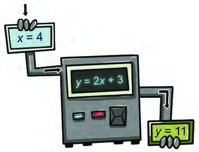
• Linear Expression Machine Example: $2x + 3$

  • Input $x = 4 \implies 2(4) + 3 = 11$

  • Input $x = -6 \implies 2(-6) + 3 = -9$

• Function Classification Comparison:

  • $2x + 3$ is a linear function.

  • $10x - x^2$ (from Example 3) is a quadratic function.

  • Evaluation of $10x - x^2$ at $x = 6\,\text{cm}$:     $\text{Area} = 10(6) - (6)^2 = 60 - 36 = 24\,\text{cm}^2$

Exercise Set 2.2 Solutions

• 1. Value of linear polynomial $5x - 3$:

  • (i) $x = 0 \implies 5(0) - 3 = -3$

  • (ii) $x = -1 \implies 5(-1) - 3 = -8$

  • (iii) $x = 2 \implies 5(2) - 3 = 7$

• 2. Value of quadratic polynomial $7s^2 - 4s + 6$:

  • (i) $s = 0 \implies 7(0)^2 - 4(0) + 6 = 6$

  • (ii) $s = -3 \implies 7(-3)^2 - 4(-3) + 6 = 7(9) + 12 + 6 = 63 + 18 = 81$

  • (iii) $s = 4 \implies 7(4)^2 - 4(4) + 6 = 7(16) - 16 + 6 = 112 - 10 = 102$

• 3. Salil's and Mother's Ages:

  • Let Salil's present age be $x\,\text{years}$. Mother's age = $3x\,\text{years}$.

  • Ages after $5\,\text{years}$: Salil = $x + 5$, Mother = $3x + 5$

  • Equation:     $(x + 5) + (3x + 5) = 70 \implies 4x + 10 = 70 \implies 4x = 60 \implies x = 15$

  • Present Ages: Salil = $15\,\text{years}$, Mother = $45\,\text{years}$.

• 4. Two Positive Integers in Ratio $2:5$ with Difference $63$:

  • Let the integers be $2x$ and $5x$

  • Equation:     $5x - 2x = 63 \implies 3x = 63 \implies x = 21$

  • Integers: $2(21) = 42$ and $5(21) = 105$

• 5. Ruby's Coin Breakdown:

  • Let the number of five-rupee coins be $x$. Number of two-rupee coins = $3x$

  • Total monetary value equation:     $5(x) + 2(3x) = 88 \implies 5x + 6x = 88 \implies 11x = 88 \implies x = 8$

  • Coin counts: Five-rupee coins = $8$, Two-rupee coins = $24$. Total coins = $32$

• 6. Cutting a Fence of $300\,\text{feet}$:

  • Let shorter piece = $x\,\text{feet}$. Longer piece = $4x\,\text{feet}$.

  • Equation:     $x + 4x = 300 \implies 5x = 300 \implies x = 60$

  • Piece lengths: Shorter piece = $60\,\text{feet}$, Longer piece = $240\,\text{feet}$.

• 7. Dimensions of Rectangle with Perimeter $24\,\text{cm}$:

  • Let width = $w\,\text{cm}$. Length = $(2w + 3)\,\text{cm}$.

  • Perimeter formula:     $2(l + w) = 24 \implies 2(2w + 3 + w) = 24 \implies 2(3w + 3) = 24 \implies 6w + 6 = 24$     $6w = 18 \implies w = 3\,\text{cm}$

  • Length $l = 2(3) + 3 = 9\,\text{cm}$.

Analyzing Linear Patterns and Sequences

• A linear pattern is a sequence of numbers in which the difference between consecutive terms is constant.

Pattern Analysis: Growing Square Tile Sequence

• Figure 2.4 illustrates a growing pattern of square tiles:

  • Stage 1: $1$ tile

  • Stage 2: $3$ tiles

  • Stage 3: $5$ tiles

  • Stage 4: $7$ tiles

  • Stage 5: $9$ tiles

  • Stage 6: $11$ tiles

  • Stage 7: $13$ tiles

• General Term Formula: At Stage $n$, the number of tiles is one less than twice the stage number:   $\text{Tiles at Stage } n = 2n - 1$

• Pattern Properties:

  • Degree of $2n - 1$: $1$ (Linear polynomial).

  • Common difference between consecutive terms: $2$

• Specific Term Evaluations using $2n - 1$:

  • 15th Stage: $2(15) - 1 = 29\,\text{tiles}$

  • 26th Stage: $2(26) - 1 = 51\,\text{tiles}$

  • Stage with 21 tiles: $2n - 1 = 21 \implies 2n = 22 \implies n = 11\,\text{th stage}$

  • Stage with 47 tiles: $2n - 1 = 47 \implies 2n = 48 \implies n = 24\,\text{th stage}$

Linear Patterns in Daily Contexts

• Example 7: Daily Pocket Money Spending

  • Initial money = $\text{₹}100$. Daily spending = $\text{₹}5$

  • Remaining money table:

  • Day 0: $\text{₹}100$

  • Day 1: $100 - 1(5) = \text{₹}95$

  • Day 2: $100 - 2(5) = \text{₹}90$

  • Day 3: $100 - 3(5) = \text{₹}85$

  • Day 4: $100 - 4(5) = \text{₹}80$

  • Expression for Day $n$: $100 - 5n$

  • Days to reach $\text{₹}40$ balance:     $100 - 5n = 40 \implies 5n = 60 \implies n = 12\,\text{days}$

  • Amount left on 15th day: $100 - 5(15) = 100 - 75 = \text{₹}25$

  • Days to spend entire amount ($\text{₹}0$): $100 - 5n = 0 \implies n = 20\,\text{days}$

• Example 8: Auto-Rickshaw Fare Structure

  • Base fare for initial $2\,\text{km}$ = $\text{₹}25$

  • Additional rate beyond $2\,\text{km}$ = $\text{₹}15\,\text{per km}$.

  • Fare Table:

  • Distance $1\,\text{km}$: $\text{₹}25$

  • Distance $2\,\text{km}$: $\text{₹}25$

  • Distance $3\,\text{km}$: $25 + 1(15) = \text{₹}40$

  • Distance $4\,\text{km}$: $25 + 2(15) = \text{₹}55$

  • Distance $5\,\text{km}$: $25 + 3(15) = \text{₹}70$

  • Distance $6\,\text{km}$: $25 + 4(15) = \text{₹}85$

  • Expression for distance $n \ge 2\,\text{km}$:     $\text{Fare} = 25 + 15(n - 2) = 15n - 5$

  • Total fare for $10\,\text{km}$ journey:     $\text{Fare} = 15(10) - 5 = \text{₹}145$

  • Distance for a fare of $\text{₹}130$:     $15n - 5 = 130 \implies 15n = 135 \implies n = 9\,\text{km}$

Exercise Set 2.3 Solutions

• 1. Savings Account Growth:

  • Initial balance = $\text{₹}500$, monthly addition = $\text{₹}150$

  • End of Month 1 = $\text{₹}650$, Month 2 = $\text{₹}800$, Month 3 = $\text{₹}950$

  • Linear expression for $n$-th month:     $\text{Amount} = 500 + 150n$

• 2. Rally Dropout Rate:

  • Initial members = $120$, dropout rate = $9\,\text{members/hour}$.

  • Members after 1 hour = $111$, 2 hours = $102$, 3 hours = $93$

  • Linear expression for $n$-th hour:     $\text{Remaining Members} = 120 - 9n$

• 3. Rectangle Area with Fixed Length ($13\,\text{cm}$):

  • (i) Breadth $12\,\text{cm} \implies \text{Area} = 13 \times 12 = 156\,\text{cm}^2$

  • (ii) Breadth $10\,\text{cm} \implies \text{Area} = 13 \times 10 = 130\,\text{cm}^2$

  • (iii) Breadth $8\,\text{cm} \implies \text{Area} = 13 \times 8 = 104\,\text{cm}^2$

  • Linear pattern for breadth $b$: $\text{Area} = 13b$

• 4. Volume of Rectangular Box ($l = 7\,\text{cm}, b = 11\,\text{cm}$):

  • Base Area = $7 \times 11 = 77\,\text{cm}^2$

  • (i) Height $5\,\text{cm} \implies \text{Volume} = 77 \times 5 = 385\,\text{cm}^3$

  • (ii) Height $9\,\text{cm} \implies \text{Volume} = 77 \times 9 = 693\,\text{cm}^3$

  • (iii) Height $13\,\text{cm} \implies \text{Volume} = 77 \times 13 = 1001\,\text{cm}^3$

  • Linear pattern for height $h$: $\text{Volume} = 77h$

• 5. Reading Progress:

  • Total pages = $500$, daily reading = $20\,\text{pages}$.

  • Linear pattern after $d\,\text{days}$: $\text{Pages Left} = 500 - 20d$

  • Pages left after 15 days: $500 - 20(15) = 200\,\text{pages}$.

Principles of Linear Growth and Linear Decay

• Linear Growth: A pattern where a quantity increases by a constant amount over equal intervals. Graphically represented by a line with a positive slope.

• Linear Decay: A pattern where a quantity decreases by a constant amount over equal intervals. Graphically represented by a line with a negative slope.

Detailed Models of Growth and Decay

• Example 9: Travel Cost Model (Linear Growth)

  • Cost equation: $C(d) = 100 + 60d$, where $C$ is total cost in Rupees and $d$ is distance in km.

  • Table of Values:

  • $d = 0\,\text{km} \implies \text{₹}100$

  • $d = 1\,\text{km} \implies \text{₹}160$

  • $d = 2\,\text{km} \implies \text{₹}220$

  • $d = 3\,\text{km} \implies \text{₹}280$

  • $d = 4\,\text{km} \implies \text{₹}340$

  • $d = 5\,\text{km} \implies \text{₹}400$

  • Growth Rate: Cost increases by a constant rate of $\text{₹}60\,\text{per km}$.

  • Cost for $15\,\text{km}$ journey: $C(15) = 100 + 60(15) = \text{₹}1000$

  • Distance for $\text{₹}700$ budget: $100 + 60d = 700 \implies 60d = 600 \implies d = 10\,\text{km}$.

• Example 10: Water Tank Evaporation Model (Linear Decay)

  • Height equation: $h(t) = 3 - 0.5t$, where $h$ is height in metres and $t$ is time in months.

  • Table of Values:

  • Month $0 \implies 3\,\text{m}$

  • Month $1 \implies 2.5\,\text{m}$

  • Month $2 \implies 2\,\text{m}$

  • Month $3 \implies 1.5\,\text{m}$

  • Month $4 \implies 1\,\text{m}$

  • Decay Rate: Height decreases by a constant rate of $0.5\,\text{m per month}$.

  • Water height at 5 months: $h(5) = 3 - 0.5(5) = 0.5\,\text{m}$.

Exercise Set 2.4 Solutions

• 1. Plant Height Growth:

  • Initial height = $1.75\,\text{feet}$, growth rate = $0.5\,\text{feet/month}$.

  • (i) Height after 7 months: $1.75 + 0.5(7) = 5.25\,\text{feet}$.

  • (ii) Table of values for $t \in [0, 10]$:

  • $t = 0 \to 1.75\,\text{ft}$

  • $t = 1 \to 2.25\,\text{ft}$

  • $t = 2 \to 2.75\,\text{ft}$

  • $t = 3 \to 3.25\,\text{ft}$

  • $t = 4 \to 3.75\,\text{ft}$

  • $t = 5 \to 4.25\,\text{ft}$

  • $t = 6 \to 4.75\,\text{ft}$

  • $t = 7 \to 5.25\,\text{ft}$

  • $t = 8 \to 5.75\,\text{ft}$

  • $t = 9 \to 6.25\,\text{ft}$

  • $t = 10 \to 6.75\,\text{ft}$

  • (iii) Relationship equation: $h(t) = 1.75 + 0.5t$. Represents linear growth because height increases by a constant positive value ($0.5\,\text{ft}$) for equal monthly time intervals.

• 2. Mobile Phone Value Depreciation:

  • Initial cost = $\text{₹}10000$, annual depreciation = $\text{₹}800\,\text{per year}$.

  • (i) Value after 3 years: $10000 - 800(3) = \text{₹}7600$

  • (ii) Table of values for $t \in [0, 8]$:

  • $t = 0 \to \text{₹}10000$

  • $t = 1 \to \text{₹}9200$

  • $t = 2 \to \text{₹}8400$

  • $t = 3 \to \text{₹}7600$

  • $t = 4 \to \text{₹}6800$

  • $t = 5 \to \text{₹}6000$

  • $t = 6 \to \text{₹}5200$

  • $t = 7 \to \text{₹}4400$

  • $t = 8 \to \text{₹}3600$

  • (iii) Relationship equation: $v(t) = 10000 - 800t$. Represents linear decay because value decreases by a constant amount ($\text{₹}800$) every year.

• 3. Village Population Expansion:

  • Initial population = $750$, annual inward migration = $50\,\text{people/year}$.

  • (i) Population after 6 years: $750 + 50(6) = 1050$

  • (ii) Table of values for $t \in [0, 10]$:

  • $t = 0 \to 750$

  • $t = 1 \to 800$

  • $t = 2 \to 850$

  • $t = 3 \to 900$

  • $t = 4 \to 950$

  • $t = 5 \to 1000$

  • $t = 6 \to 1050$

  • $t = 7 \to 1100$

  • $t = 8 \to 1150$

  • $t = 9 \to 1200$

  • $t = 10 \to 1250$

  • (iii) Relationship equation: $P(t) = 750 + 50t$. Represents linear growth because the population increases by a constant amount ($50$) each year.

• 4. Prepaid Balance Exhaustion:

  • Initial balance = $\text{₹}600$, daily usage = $\text{₹}15\,\text{per day}$.

  • (i) Equation: $b(x) = 600 - 15x$. Represents linear decay because the remaining balance decreases by a fixed amount ($\text{₹}15$) daily.

  • (ii) Days until balance runs out ($b(x) = 0$):     $600 - 15x = 0 \implies 15x = 600 \implies x = 40\,\text{days}$

  • (iii) Table of values for $x \in [1, 10]$:

  • Day $1 \to \text{₹}585$

  • Day $2 \to \text{₹}570$

  • Day $3 \to \text{₹}555$

  • Day $4 \to \text{₹}540$

  • Day $5 \to \text{₹}525$

  • Day $6 \to \text{₹}510$

  • Day $7 \to \text{₹}495$

  • Day $8 \to \text{₹}480$

  • Day $9 \to \text{₹}465$

  • Day $10 \to \text{₹}450$

Formulation of Linear Relationships

• A linear relationship between two variables $x$ and $y$ is expressed in the standard form:   $y = ax + b$   where $a$ is the rate of change (slope) and $b$ is the initial/fixed constant (y-intercept).

Solving for Parameters in Linear Relationships

• Example 11: Internet Data Billing Structure

  • Model equation: $y = ax + b$, where $x$ is data used in GB and $y$ is total monthly bill in Rupees.

  • Data Points:

  • Usage $10\,\text{GB} \implies \text{Bill } \text{₹}350 \implies 350 = 10a + b$

  • Usage $20\,\text{GB} \implies \text{Bill } \text{₹}550 \implies 550 = 20a + b$

  • System Solution:

  1. Express $b$ from first equation: $b = 350 - 10a$

  2. Substitute into second equation:        $550 = 20a + (350 - 10a) \implies 550 = 10a + 350 \implies 10a = 200 \implies a = 20$

  3. Calculate $b$:        $b = 350 - 10(20) = 150$

  • Resulting Relationship: $y = 20x + 150$

  • Meaning of Parameters:

  • $a = 20$ represents the variable charge per GB of data used ($\text{₹}20/\text{GB}$).

  • $b = 150$ represents the fixed monthly subscription fee ($\text{₹}150$).

Exercise Set 2.5 Solutions

• 1. Online Learning Platform Fee:

  • Model: $y = ax + b$

  • Points: $(10, 400)$ and $(14, 500)$

  • Equations:     $10a + b = 400$     $14a + b = 500$

  • Subtracting equations:     $4a = 100 \implies a = 25$     $b = 400 - 10(25) = 150$

  • Parameters: $a = 25$, $b = 150$ (Relationship: $y = 25x + 150$).

• 2. Gym Badminton Court Fee:

  • Model: $y = ax + b$

  • Points: $(10, 800)$ and $(15, 1100)$

  • Equations:     $10a + b = 800$     $15a + b = 1100$

  • Subtracting equations:     $5a = 300 \implies a = 60$     $b = 800 - 10(60) = 200$

  • Parameters: $a = 60$, $b = 200$ (Relationship: $y = 60x + 200$).

• 3. Celsius and Fahrenheit Temperature Conversion:

  • Model: $^\circ\text{C} = a\,^\circ\text{F} + b$

  • Freezing Point: $0^\circ\text{C} = 32^\circ\text{F} \implies 0 = 32a + b \implies b = -32a$

  • Boiling Point: $100^\circ\text{C} = 212^\circ\text{F} \implies 100 = 212a + b$

  • Substituting $b = -32a$:     $100 = 212a - 32a = 180a \implies a = \frac{100}{180} = \frac{5}{9}$     $b = -32 \left(\frac{5}{9}\right) = -\frac{160}{9}$

  • Parameters: $a = \frac{5}{9}$, $b = -\frac{160}{9}$

  • Full Linear Equation: $^\circ\text{C} = \frac{5}{9}(^\circ\text{F} - 32)$

Graphical Representation of Linear Relationships

• The graph of any linear equation $y = ax + b$ on a coordinate plane is a straight line.

• A minimum of two distinct points is required to plot a straight line.

Graphing Techniques and Point Verification

• Plotting $y = 2x + 1$:

  • Point A ($x = 0$): $y = 2(0) + 1 = 1 \implies A(0, 1)$

  • Point B ($x = 3$): $y = 2(3) + 1 = 7 \implies B(3, 7)$

• Completed Coordinate Table for $y = 2x + 1$:

  • $x = 1 \implies y = 2(1) + 1 = 3 \implies (1, 3)$

  • $x = 2 \implies y = 2(2) + 1 = 5 \implies (2, 5)$

  • $x = 5 \implies y = 2(5) + 1 = 11 \implies (5, 11)$

  • $x = 7 \implies y = 2(7) + 1 = 15 \implies (7, 15)$

  • $x = 9 \implies y = 2(9) + 1 = 19 \implies (9, 19)$

  • $x = 12 \implies y = 2(12) + 1 = 25 \implies (12, 25)$

  • $x = 20 \implies y = 20(2) + 1 = 41 \implies (20, 41)$

• Point Verification Rule: A point $(x_0, y_0)$ lies on a line if and only if its coordinates satisfy the linear equation $y_0 = a x_0 + b$

  • Verification for $(7, 15)$: $2(7) + 1 = 14 + 1 = 15$, confirming it lies on $y = 2x + 1$

• Example 12: Graphing Positive Slope Line $y = 3x$

  • Coordinates: $(-1, -3)$, $(0, 0)$, $(1, 3)$, $(3, 9)$, $(4, 12)$.

  • Observed Rule: Each y-coordinate is three times the x-coordinate ($y = 3x$).

• Example 13: Graphing Negative Slope Line $y = -2x$

  • Coordinates: $(-3, 6)$, $(-2, 4)$, $(0, 0)$, $(1, -2)$, $(2, -4)$, $(3, -6)$.

  • Observed Rule: Each y-coordinate is $-2$ times the x-coordinate ($y = -2x$).

Influence of Slope ($a$) on Direct Proportionality Lines ($y = ax$)

• Equations: $y = \frac{1}{2}x$, $y = x$, $y = 2x$

• Key Graphical Characteristics:

  • Every line of the form $y = ax$ passes through the origin $(0, 0)$.

  • When a > 1, the line is steeper than $y = x$

  • When a < 1, the line is less steep than $y = x$

  • The coefficient $a$ represents the slope (steepness) of the line.

  • Positive slopes represent linear growth; negative slopes represent linear decay.

• Negative Slope Lines ($y = -ax$):

  • Equations: $y = -\frac{1}{3}x$, $y = -x$, $y = -3x$

  • Slope direction: Lines slant downwards from left to right.

  • Graph Comparison ($y = 3x + 1$ vs $y = -3x + 1$): $y = 3x + 1$ slants upwards (positive slope 3, linear growth), whereas $y = -3x + 1$ slants downwards (negative slope -3, linear decay). Both cross the y-axis at $(0, 1)$.

Influence of y-Intercept ($b$) and Parallel Lines

• Equations: $y = 2x - 1$, $y = 2x + 1$, $y = 2x + 5$

  • Slope $a = 2$ is identical for all three lines.

  • Parallel Lines Principle: Lines with equal slopes but different y-intercepts are parallel to each other.

• y-Intercept Definition: The point where a straight line crosses the y-axis is $(0, b)$. The constant $b$ is called the y-intercept.

  • $y = 2x + 5$ cuts the y-axis at $A(0, 5)$ (y-intercept = $5$).

  • $y = x + 3$ cuts the y-axis at $B(0, 3)$ (y-intercept = $3$).

  • $y = 3x - 2$ cuts the y-axis at $C(0, -2)$ (y-intercept = $-2$).

Summary of Graphical Rules for $y = ax + b$

• In $y = ax + b$, $a$ represents slope, and $b$ represents y-intercept.

• Changing $a$ while keeping $b$ fixed rotates the line around $(0, b)$, altering its steepness.

• Changing $b$ while keeping $a$ fixed shifts the line vertically, maintaining parallelism with the original line.

Exercise Set 2.6 Solutions

• 1. Graph Families:

  • (i) $y = 4x, y = 2x, y = x$: All pass through $(0, 0)$. Steeper slope for larger $a$

  • (ii) $y = -6x, y = -3x, y = -x$: All pass through $(0, 0)$. Downward slanting; steeper negative slope for larger magnitude of $a$

  • (iii) $y = 5x, y = -5x$: Pass through origin $(0, 0)$; reflections of each other across the y-axis.

  • (iv) $y = 3x - 1, y = 3x, y = 3x + 1$: Parallel lines with slope $a = 3$ and y-intercepts $-1, 0, 1$

  • (v) $y = -2x - 3, y = -2x, y = 2x + 3$: $y = -2x - 3$ and $y = -2x$ are parallel with slope $-2$; $y = 2x + 3$ has positive slope $2$ and y-intercept $3$

Comprehensive Chapter Exercises and Solutions

• 1. Polynomial Construction:

  • Degree 3 polynomial in variable $x$ with $x^2$ coefficient $-7$:     $p(x) = x^3 - 7x^2 + 4x + 2$

• 2. Polynomial Evaluations:

  • (i) $5x^2 - 3x + 7$ at $x = 1$:     $5(1)^2 - 3(1) + 7 = 5 - 3 + 7 = 9$

  • (ii) $4t^3 - t^2 + 6$ at $t = a$:     $4a^3 - a^2 + 6$

• 3. Number Problem:

  • Let the number be $x$

  • Equation:     $\frac{5}{2}x + \frac{2}{3} = -\frac{7}{12}$

  • Solving for $x$:     $\frac{5}{2}x = -\frac{7}{12} - \frac{8}{12} = -\frac{15}{12} = -\frac{5}{4}$     $x = -\frac{5}{4} \times \frac{2}{5} = -\frac{1}{2}$

• 4. Positive Number Comparison:

  • Let one number be $y$ and the positive number be $5y$

  • Adding $21$ to both yields $5y + 21$ and $y + 21$

  • Equation:     $5y + 21 = 2(y + 21) \implies 5y + 21 = 2y + 42 \implies 3y = 21 \implies y = 7$

  • The numbers are $7$ and $35$

• 5. Savings Pattern:

  • Initial amount = $\text{₹}800$, monthly savings = $\text{₹}250$

  • Pattern expression for $m$ months: $\text{Amount} = 800 + 250m$

  • (i) After 6 months: $800 + 250(6) = 800 + 1500 = \text{₹}2300$

  • (ii) After 2 years ($24\,\text{months}$): $800 + 250(24) = 800 + 6000 = \text{₹}6800$

• 6. Two-Digit Number Problem:

  • Digits differ by 3.

  • Let tens digit = $x$ and units digit = $x + 3$

  • Original number = $10x + (x + 3) = 11x + 3$

  • Interchanged number = $10(x + 3) + x = 11x + 30$

  • Sum equation:     $(11x + 3) + (11x + 30) = 143 \implies 22x + 33 = 143 \implies 22x = 110 \implies x = 5$

  • Digits are $5$ and $8$

  • Both possible numbers are $58$ and $85$

• 7. Line Properties and Parallel Line Identification:

  • (i) $y = -3x + 4$ $\implies$ Slope $a = -3$, y-intercept $b = 4$, y-axis point $(0, 4)$.

  • (ii) $2y = 4x + 7 \implies y = 2x + \frac{7}{2}$ $\implies$ Slope $a = 2$, y-intercept $b = \frac{7}{2}$, y-axis point $(0, 3.5)$.

  • (iii) $5y = 6x - 10 \implies y = \frac{6}{5}x - 2$ $\implies$ Slope $a = \frac{6}{5}$, y-intercept $b = -2$, y-axis point $(0, -2)$.

  • (iv) $3y = 6x - 11 \implies y = 2x - \frac{11}{3}$ $\implies$ Slope $a = 2$, y-intercept $b = -\frac{11}{3}$, y-axis point $\left(0, -\frac{11}{3}\right)$.

  • Parallel Lines: Lines (ii) and (iv) are parallel because both have an identical slope of $a = 2$

• 8. Kelvin to Fahrenheit Conversion:

  • Equation: $y = \frac{9}{5}(x - 273) + 32$

  • (i) Temperature at $x = 313\,\text{K}$:     $y = \frac{9}{5}(313 - 273) + 32 = \frac{9}{5}(40) + 32 = 72 + 32 = 104^\circ\text{F}$

  • (ii) Temperature at $y = 158^\circ\text{F}$:     $158 = \frac{9}{5}(x - 273) + 32 \implies 126 = \frac{9}{5}(x - 273) \implies x - 273 = 70 \implies x = 343\,\text{K}$

• 9. Work Done by Constant Force:

  • Equation with force $F = 3\,\text{units}$: $w = 3d$

  • Work done when distance $d = 2\,\text{units}$:     $w = 3(2) = 6\,\text{units}$

• 10. Determining Linear Polynomial from Points:

  • Graph passes through $(1, 5)$ and $(3, 11)$.

  • Let $p(x) = ax + b$

  • Equations:     $a + b = 5$     $3a + b = 11$

  • Subtracting equations:     $2a = 6 \implies a = 3$     $b = 5 - 3 = 2$

  • (i) Polynomial: $p(x) = 3x + 2$

  • (ii) Axis Intercepts:

  • y-axis ($x = 0$): $(0, 2)$

  • x-axis ($p(x) = 0$): $3x + 2 = 0 \implies x = -\frac{2}{3} \implies \left(-\frac{2}{3}, 0\right)$

• 11. System of Two Linear Polynomials:

  • Let $p(x) = ax + b$ and $q(x) = cx + d$

  • Condition (i): $p(0) = 5 \implies b = 5$

  • Condition (iii): $p(x) + q(x) = 6x + 4 \implies (a + c)x + (5 + d) = 6x + 4$

  • $a + c = 6$

  • $5 + d = 4 \implies d = -1$

  • Condition (ii): $p(x) - q(x) = (a - c)x + (5 - (-1)) = (a - c)x + 6$ cuts x-axis at $(3, 0)$:     $(a - c)(3) + 6 = 0 \implies 3(a - c) = -6 \implies a - c = -2$

  • Solving for $a$ and $c$:

  • Add $a + c = 6$ and $a - c = -2 \implies 2a = 4 \implies a = 2$

  • $c = 6 - 2 = 4$

  • Resulting Polynomials: $p(x) = 2x + 5$ and $q(x) = 4x - 1$

• 12. Hexagon Matchstick Pattern:

  • Stage 1: $1$ hexagon = $6$ matchsticks

  • Stage 2: $2$ joined hexagons = $11$ matchsticks

  • Stage 3: $3$ joined hexagons = $16$ matchsticks

  • (i) Next two stages: Stage 4 requires $21$ matchsticks; Stage 5 requires $26$ matchsticks.

  • (ii) Matchstick Table:

  • Stage 1: $6$

  • Stage 2: $11$

  • Stage 3: $16$

  • Stage 4: $21$

  • Stage 5: $26$

  • Stage $n$: $5n + 1$

  • (iii) Rule for $n$-th stage: $5n + 1$

  • (iv) Matchsticks for 15th stage: $5(15) + 1 = 76\,\text{matchsticks}$

  • (v) Can 200 matchsticks form a stage?     $5n + 1 = 200 \implies 5n = 199 \implies n = 39.8$     Since $n$ must be an integer, 200 matchsticks cannot form a stage in this pattern.

• 13. Parallel Linear Polynomials:

  • $p(x) = ax + b$ passes through $(2, 3)$ and $(6, 11)$:     $\text{Slope } a = \frac{11 - 3}{6 - 2} = \frac{8}{4} = 2$     $3 = 2(2) + b \implies b = -1 \implies p(x) = 2x - 1$

  • $q(x) = cx + d$ is parallel to $p(x) \implies c = a = 2$

  • $q(x)$ passes through $(4, -1)$:     $-1 = 2(4) + d \implies -1 = 8 + d \implies d = -9 \implies q(x) = 2x - 9$

  • x-axis Intercepts ($y = 0$):

  • $p(x) = 0 \implies 2x - 1 = 0 \implies x = \frac{1}{2} \implies \left(\frac{1}{2}, 0\right)$

  • $q(x) = 0 \implies 2x - 9 = 0 \implies x = \frac{9}{2} \implies \left(\frac{9}{2}, 0\right)$

• 14. Shared Feature of $f(x) = ax + a$, a > 0:

  • Factoring expression: $f(x) = a(x + 1)$

  • Evaluating at $x = -1$: $f(-1) = a(-1 + 1) = 0$ for all a > 0

  • Shared Characteristics: All functions in this family pass through the point $(-1, 0)$ on the x-axis (x-intercept is $-1$) and have a y-intercept equal to their slope $a$