Understanding the Fourier Transfrom

Fundamental Principles

Part 1 (sine waves only)

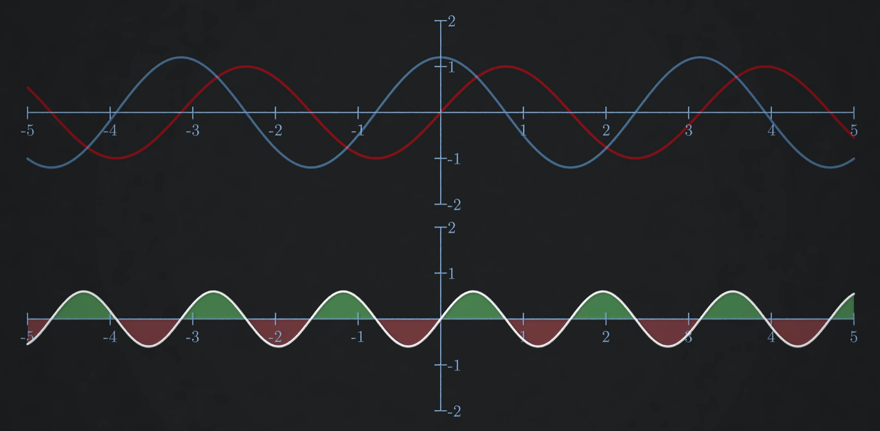
If you want to know how much of a particular sine wave (with phase zero) contributes to a signal, just multiply the signal by the sine wave at each point, and then add up the area under the curve. To note, we are only considering a standard sine wave with no phase shift (we only choose the frequency).

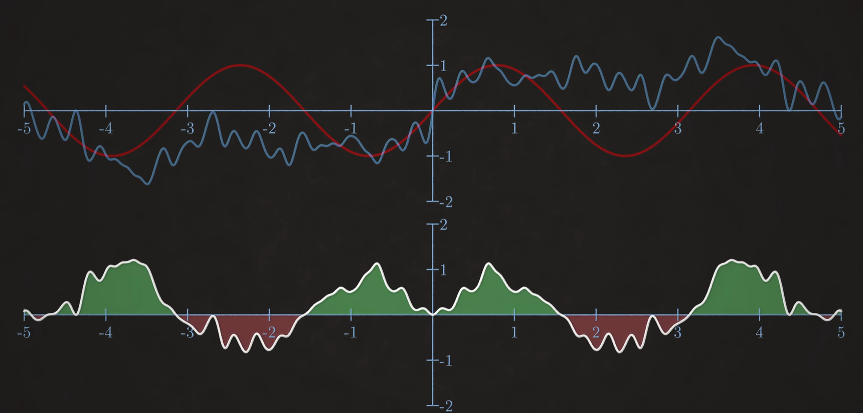
The sine wave we multiply the signal with has an amplitude of just one. The summed green area would tell us what amplitude this sine wave actually contributes.

Question. If the sine wave and signal match exactly with only green area, shouldn’t integral sum to infinity? Answer: You’re right. FT only converges for finite signals.

Part 2 (cosine waves)

So far, we’ve only multiplied by sine waves. However, this wouldn’t be complete.

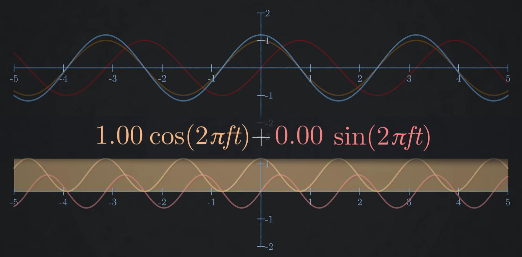
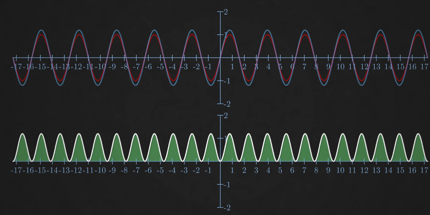
This means we have to multiply the signal by a sine wave and a cosine wave, and find amplitude contributions for each. The above diagram shows a cosine signal (blue) being multiplied by a sine and cosine signal (yellow and red). The red wave results to zero, meaning no contribution from the sine wave, and the yellow wave makes full contribution. This is reflected in the equation, with amplitude 1 and 0.

Now what if the blue signal is shifted?

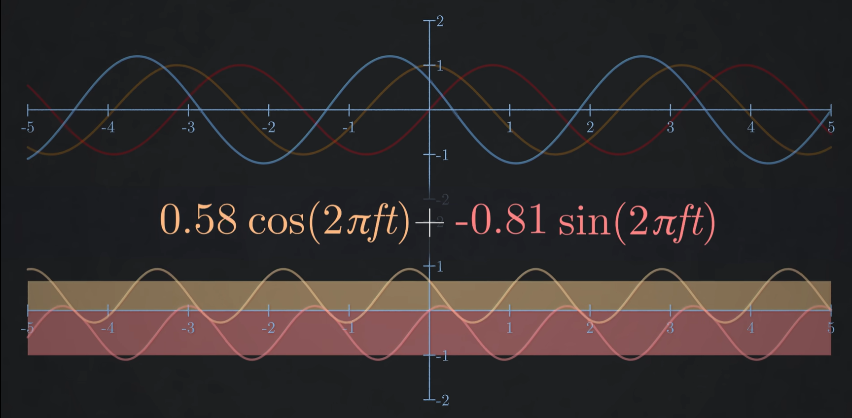
Both the red sine wave and yellow cosine wave make contributions. The ratio of their contributions is the phase of the original signal.

Remember the identity:

$a \cos(x) + b \sin(x) = R \sin(x + \theta)$

where:

- $R = \sqrt{a^2 + b^2}$

- $\theta = \tan^{-1}\left(\frac{a}{b}\right)$

Multiplying by both a sine and cosine wave, we can capture the contribution of a sinusoidal wave of any phase.

To create the frequency spectrum for this example, we simply take $R$ as the amplitude at a frequency $f$. This also means that two identical signals with different phases would have the same frequency spectrum, but have different phase diagrams.

Final Part

The following quote is from the start of this document,

Now we can say instead, that if we want to know how much of a sine wave of a specific frequency with a phase shift is in a signal, just multiply the signal by a sine wave and a cosine wave at each point. The ratio of the contributions determines the contribution of a particular sine wave with a particular phase shift.

Quite conveniently, we have Euler’s formula:

$\cos(2\pi ft) + i\sin(2\pi ft) = e^{i2\pi ft}$

We only need to multiply the signal by an exponential, where the real part of the sum is the cosine amplitude, and the imaginary part is the sine amplitude.

Recap

• It is possible to break a signal down into a sum of sine waves, with each wave having it’s own amplitude, frequency and phase.

• We do this by first specifying a frequency of wave we want to test, then multiplying the signal by a sine and cosine of that frequency. From this, we can find the contribution of the wave and it’s phase shift.

• Consider the following formula:
  $a\cos(2\pi ft)+b\sin(2\pi ft)=R\sin(2\pi ft+\theta)$

  $a$ and $b$ are the contributions we learn from the integration sum for each wave.

  $\theta$ is the phase shift of the wave we are testing.

  $R$ is the contribution of that wave.

• We’ve now found the contribution of a specific frequency wave, as well as it’s phase. All that’s left to do is plot the contribution in a frequency spectrum.

We can derive an equation that will give us the contribution and phase of a sinusoid of any frequency $w$. We do this using…

The Fourier Transform

Continuous-Time Fourier Transform (CTFT)

Given a continuous-time signal $x(t)$:

$X(j\omega) = \int_{-\infty}^{\infty} x(t) \cdot e^{-j\omega t} \, dt$

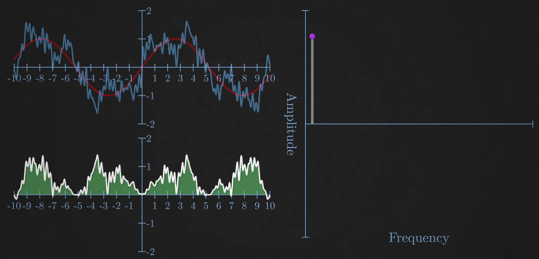
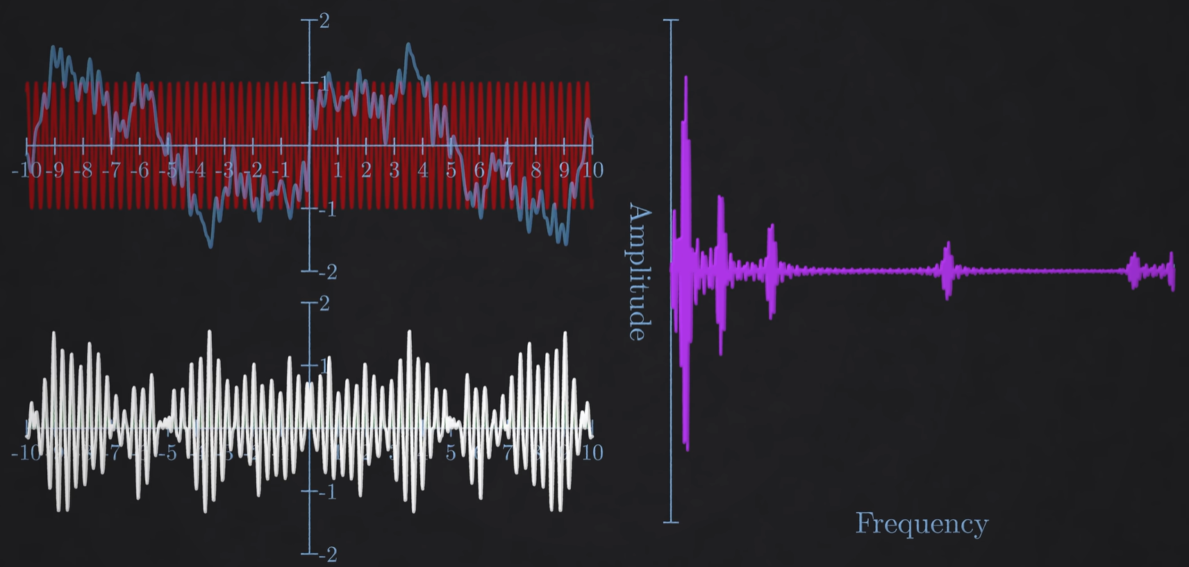
We multiply the signal by a sine and cosine of frequency $w$, and then integrate to find the contribution of a sinusoid of frequency $w$. This is exactly what we are trying to do!

Plotting the magnitude of $X(j\omega)$ gives us the frequency spectrum.

Now, what if the signal was discrete…

Discrete Time Fourier Transform

The immediate analogy for the Fourier Transform in the discrete domain is the Discrete Time Fourier Transform, where $t$ is replaced with $n$, the sample number. The output is a continuous periodic spectrum. The transform works identically to the standard Fourier, but now only multiplying and integrating over sampled points.

Discrete Time Fourier Transform:

$X(e^{j\omega})=\sum_{k=-\infty}^{\infty}x[k]e^{-j\omega k}$

• Input: Discrete-time signal, potentially of infinite length

• Output: Continuous function of frequency, defined for all $\omega \in [-\pi, \pi]$

  • The output is periodic with period

  • This is like typical sampling shown in Image Processing

Discrete Fourier Transform

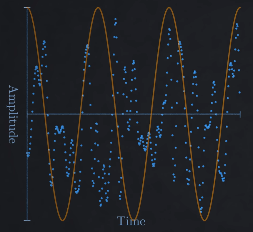
In reality, discrete signals have a finite duration. We take a different approach to computing the spectrum, treating the finite samples as periodic and representing the spectrum as a combination of harmonic frequencies.

As the samples are finite (and further considered periodic), we only need a finite number of frequencies to represent the signal. The reason why we have to consider the samples as periodic is because a finite set of frequencies will always produce a periodic signal when summed. This in contrast to the ideal frequency spectrum for an infinite signal, that would require an infinite number of frequencies to completely reconstruct.

Harmonic Frequencies

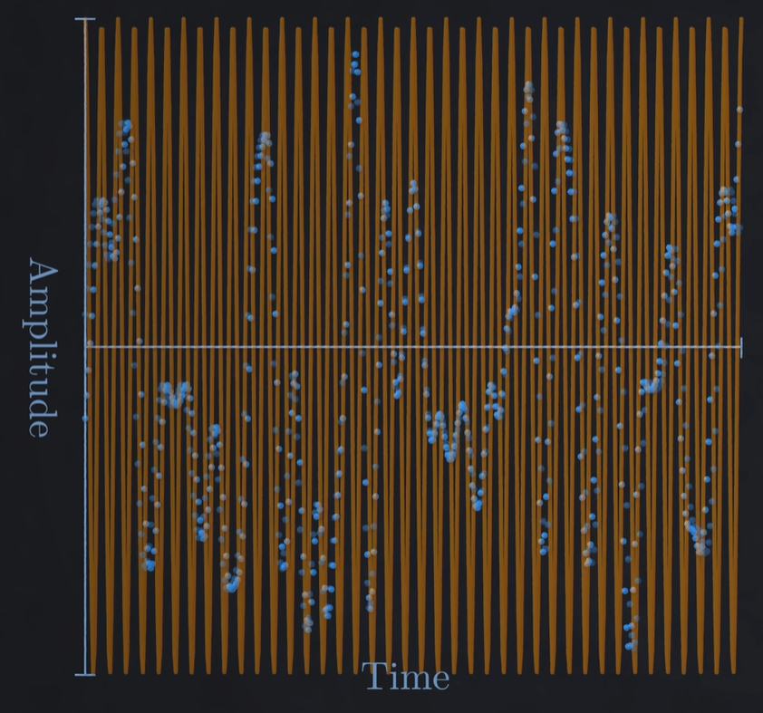
The lowest frequency measurable in a finite set of samples is the frequency equal to the duration of the signal.

Higher detectable frequencies are just integer multiples of this fundamental frequency.

The maximum measurable frequency is limited by the number of samples.

The total number of frequencies we use to represent the signal is equal to the number of samples in the signal, $N$.

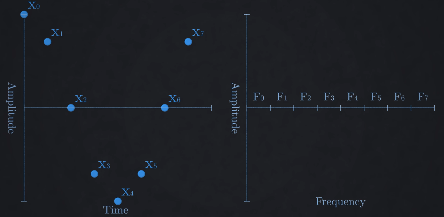
There are 8 samples in this signal, so we use 8 harmonic frequencies representing the signal.

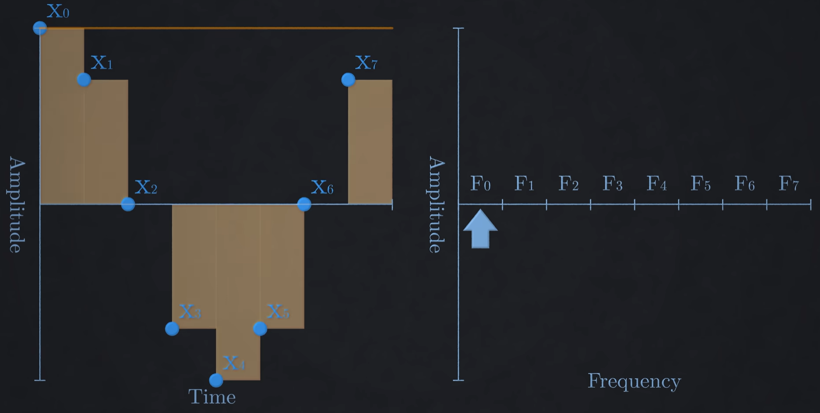
Here we multiply by the DC value (1 in this case) and then integrate. This sums to zero, so there is no DC offset/contribution.

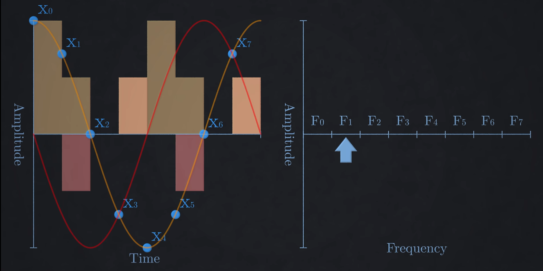
Now we look at the lowest frequency. We multiply by a sine and cosine of the same frequency and integrate to find the contribution of this frequency.

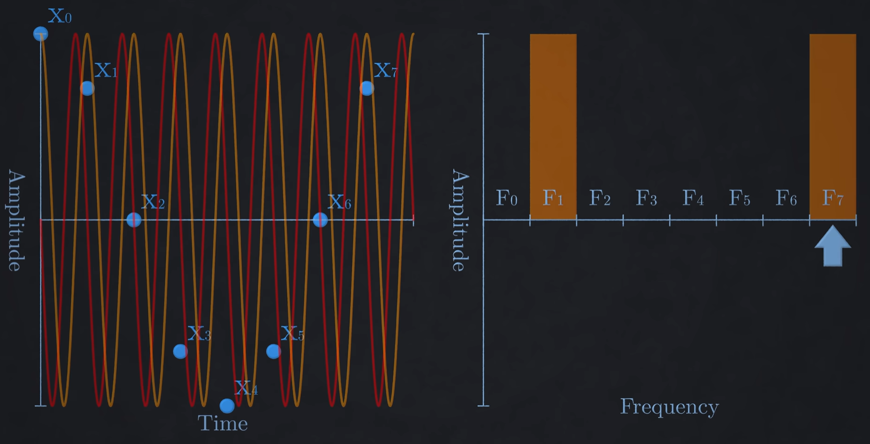
Continue doing this for each frequency multiple. Now you have the discrete frequency spectrum.

DFT Equation

Now we must represent this mathematically.

Discrete Fourier Transform:

$X[n]=\sum_{k=0}^{N-1}x[k]e^{-j2\pi\frac{n}{N}k},\quad n=0,1,...,N-1$

• Input: Finite-duration discrete-time signal of length $N$

• Output: Finite set of $N$ complex numbers representing frequency samples

  • $X[n]$, where $n = 0, 1, ..., N-1$

  • These are coefficients or contributions of the harmonic frequencies.
    

There are two indexes, $k$ and $n$:

• $k$ refers to the discrete sample in $x[k]$ and is also the discrete analogy for $t$.

  • The analogy explains why $k$ appears in the exponential. Standard form for a sinusoid:$\cos\left(wt\right)=\cos\left(2\pi ft\right)=\cos\left(2\pi\frac{t}{T}\right)=\cos\left(2\pi\cdot\underbrace{\frac{1}{N}\cdot n}_{\text{frequency }f\text{ or }\frac{1}{T}}\cdot\underbrace{k}_{\text{time }t}\right)\Rightarrow e^{-j2\pi\frac{n}{N}k}$

  • $n$ refers to the harmonic frequency/coefficient number.

For example, to find the coefficient for the second harmonic frequency, you would set $n=2$ in the equation, then sum from $k=0$ to $k=N-1$ (since we have $N$ samples and the first sample is indexed at 0).

The equation multiplies the signal by a harmonic frequency at discrete points on the wave, then integrates (sums) to find the contribution.

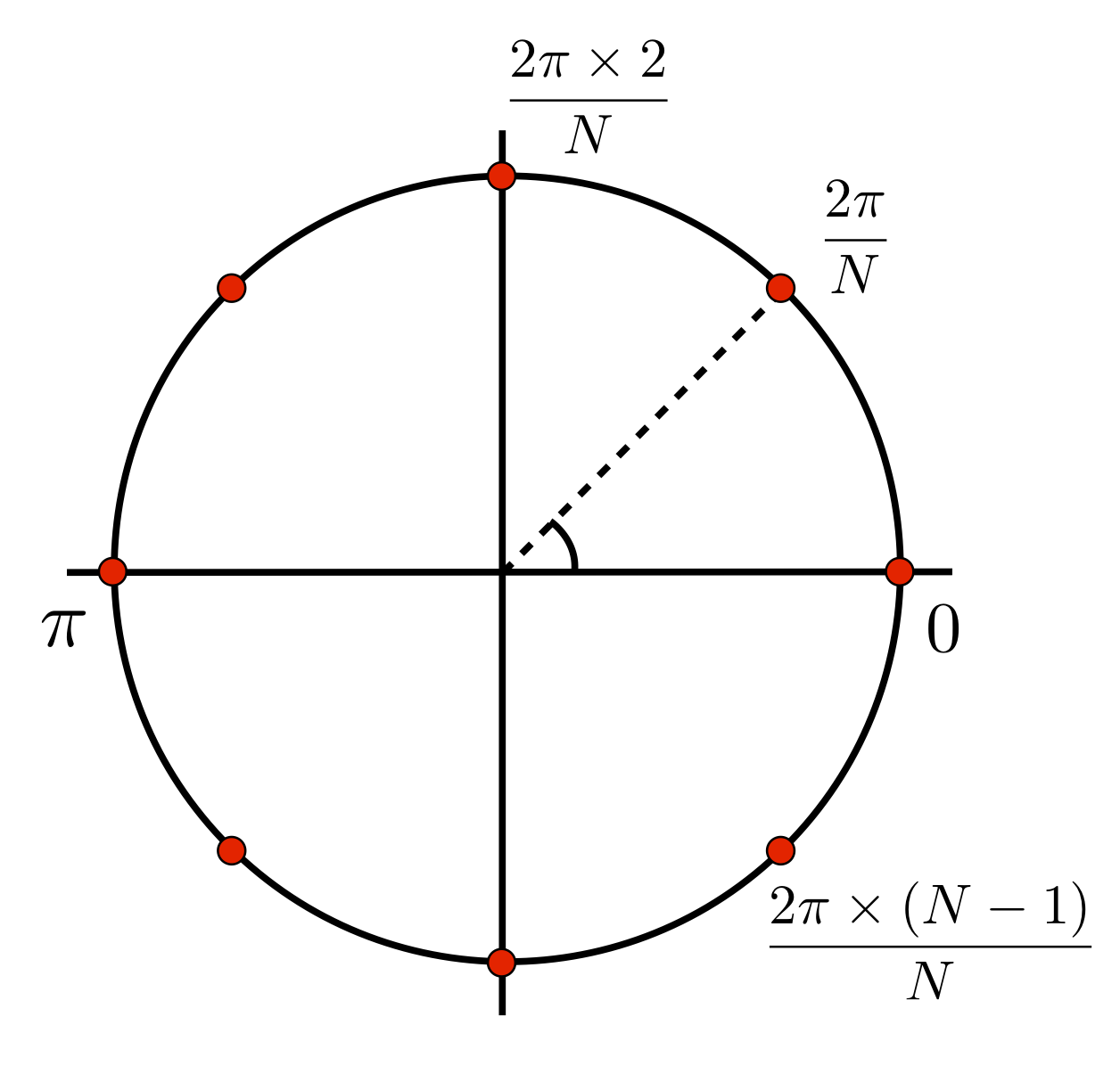
Frequency of the first harmonic is $f_1=\frac{1}{N}$, and for nth harmonic,$f_{n}=\frac{n}{N}$ , up to $N-1$ (Nth frequency would be the same as the first harmonic). These can be represented on a unit circle in angular frequency (radians), $\omega_{n}=2\pi\frac{n}{N}$.

Example

$x[k] = \{1, 2, 3, 4\}$, $N = 4$

Compute $X[0]$ (DC coefficient):

$X[0] = \sum_{k=0}^{3} x[k] \cdot e^{-j \cdot \frac{2\pi}{4} \cdot 0 \cdot k} = \sum_{k=0}^{3} x[k] \cdot 1 = 1 + 2 + 3 + 4 = 10$

Compute $X[1]$ (coefficient for first harmonic):

$X[1] = \sum_{k=0}^{3} x[k] \cdot e^{-j \cdot \frac{2\pi}{4} \cdot 1 \cdot k} = x[0] \cdot 1 + x[1] \cdot e^{-j\frac{\pi}{2}} + x[2] \cdot e^{-j\pi} + x[3] \cdot e^{-j\frac{3\pi}{2}}$

Each exponential in this sum is basically a sampled point on the harmonic we are testing. Imagine the $k$ was $t$, and the integral was with respect to $t$ , multiplying each point on the sine with the signal.

$X[1] = 1 + 2(-j) + 3(-1) + 4(j) = 1 - 2j - 3 + 4j = (-2) + 2j$

$X[1] = -2 + 2j$

Imagine the $k$ in the exponential is analogous to $t$ but only at discrete points. This is to multiply discrete points on the sinusoid with discrete signal samples.

Compute $X[2]$:

$X[2] = \sum_{k=0}^{3} x[k] \cdot e^{-j \cdot \frac{2\pi}{4} \cdot 2 \cdot k}$

We calculate each exponential term:

- $e^{-j \cdot \frac{2\pi}{4} \cdot 2 \cdot 0} = e^{0} = 1$

- $e^{-j \cdot \frac{2\pi}{4} \cdot 2 \cdot 1} = e^{-j\pi} = -1$

- $e^{-j \cdot \frac{2\pi}{4} \cdot 2 \cdot 2} = e^{-j2\pi} = 1$

- $e^{-j \cdot \frac{2\pi}{4} \cdot 2 \cdot 3} = e^{-j3\pi} = -1$

So:

$X + x + x[3](-1) = 1 - 2 + 3 - 4 = -2$

$X[2] = -2$

Compute $X[3]$:

$X[3] = \sum_{k=0}^{3} x[k] \cdot e^{-j \cdot \frac{2\pi}{4} \cdot 3 \cdot k}$

Evaluate each term:

- $e^{-j \cdot \frac{2\pi}{4} \cdot 3 \cdot 0} = e^{0} = 1$

- $e^{-j \cdot \frac{2\pi}{4} \cdot 3 \cdot 1} = e^{-j\frac{3\pi}{2}} = j$

- $e^{-j \cdot \frac{2\pi}{4} \cdot 3 \cdot 2} = e^{-j3\pi} = -1$

- $e^{-j \cdot \frac{2\pi}{4} \cdot 3 \cdot 3} = e^{-j\frac{9\pi}{2}} = -j$

Now substitute:

$X[3] = 1 + 2(j) + 3(-1) + 4(-j) = 1 + 2j - 3 - 4j = (-2) - 2j$

$X[3] = -2 - 2j$

Final DFT Result:

$X[0] = 10$

$X[1] = -2 + 2j$

$X[2] = -2$

$X[3] = -2 - 2j$

Questions

Why is the frequency spectrum of am infinite aperiodic discrete signal, continuous and periodic?

Answer: Go back to image processing and read how sampling a signal in time domain is like multiplying with a comb function, and in the frequency domain, this is like convolving with the Fourier Transform of the comb function, which repeats the spectrum.