Week 2
Goals of Psychological Research
Draw conclusions about a population based on your sample
Population: who we’re interested in (e.g., young adults between 18-25)
Sample: who we collect data from (e.g., 150 UIowa undergraduates)
Note on Symbols
(Usually) Roman letters for samples; Greek letters for populations
e.g., “x bar” is the mean of some variables in your sample
“mu” is the mean of some variable in the population
e.g., “R” is the correlation between variables in your sample
“rho” is the correlation between variables in the population
Inferential vs. Descriptive Statistics
Descriptive statistics describe (summarize) a sample
e.g., the man BDI score was 8.5
Inferential statistics attempt to extend beyond the sample
e.g., My best guess for the population mean is 8.5 … and I’m confident that it’s between 5 and 12
Inferences can be wrong (even when you do everything right)
Sampling bias and/or sampling error
Sampling Bias
Ideally, samples should be unbiased
Everyone in the population has an equal chance of recruitment
Representative: sample demographics reflect population demographics
Most common method: random sampling
In practice, more samples are biased
Not everyone in the population has equal chance of recruitment
Nonrepresentative: sample demographics don’t reflect population demographics
Most common method: Convenience sampling
Sampling bias is avoidable
Sampling Error
Random variability in a statistic from sample to sample
Can occur even after unbiased (e.g., random) sampling
Sampling error is not (entirely) avoidable
Two major implications:
Relationships in the population might not show up in a sample
Relationships in a sample might not exist in the population
The Many Methods of Hypothesis Testing
Null hypothesis significance testing (NHST)
Bayesian inference
Mixed-effects modelling
Logic of Hypothesis Testing
It’s difficult (impossible?) to improve that something is true
e.g., “BDI and HAM are related” - maybe they are related in my sample of 150 UIowa undergrads, but …
“What if you had a bigger sample?”
“What if you recruited Iowa State undergrads?”
“What if you recruited young adults who aren’t in college?”
“What if you recruited people from [Canada/Kenya/Mongolia/Australia]?”
“What about … ?”
But it’s relatively easy to disprove that something is true
e.g., “BDI and HAM are not related”
Only need one counterexample - e.g., my 150 UIowa undergrads
Instead of proving that a relationship exists, we try to disprove that it doesn’t exist
If we disprove that BDI and HAM aren’t related (e.g., by finding a significant correlation in our sample), then we have support for our hypothesis that they are related
The name for no relationship is “null hypothesis” (H0)
e.g., in correlational studies, H0 is that pyx = 0
If you reject H0, then you support an “alternative hypothesis” (H1)
e.g., in correlational studies, H1 is that pyx ! = 0
How do we reject H0?
It’s not enough to say that ryx ! = 0 (see again: sampling error)
Also need to show that ryx we obtained would be highly unlikely if pyx = 0
p Values
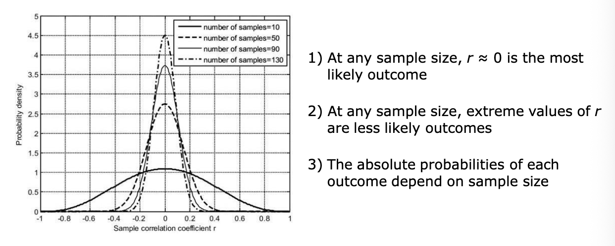
With a specified H0 and a selected sample size, you can calculate the probability of all potential outcomes in advance
(Under the assumption that H0 is true)
This is called the sampling distribution
The calculated probability of a particular, observed outcome is the p value for that outcome
More specifically: the p value is the probability of obtaining an outcome at least as extreme as your observed outcome, if H0 were true
e.g., r = 0.12, p = 0.810 means that there’s 81.0% chance of obtaining a correlation of at least 0.12 if H0 were true
P values are not the probability that your result was due to chance (we’re not assuming chance; we’re assuming H0!)
If p is sufficiently low, then we can reject H0
Because out outcome would be very unlikely if H0 were true
If p is sufficiently high, then we fail to reject (retain) H0
Because our outcome would be relatively likely even if H0 were true
We never “accept” H0 (again, it’s really hard to prove that something is true)
The cut-off is a (“alpha”), which we always set at 0.05
If p < 0.05 then we reject H0
If p >= 0.05 then we fail to reject H0
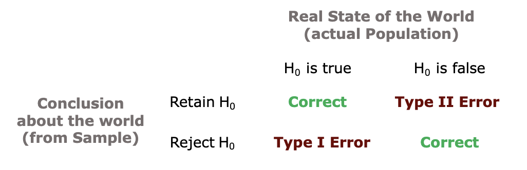
We set a really strict a (0.05) to minimize Type I errors
General agreement that it’s worse to make a Type I error than a Type II error
In theory, you could raise alpha (e.g., reject H0 if p < 0.10)
Increases risk of Type I errors, but decrease risk of Type II errors (trade-off)
In practice, this is really hard to justify (these days) and pretty much never happens (these days)
Decision Errors in Hypothesis Testing
Remember; disproving H0 is error-prone (because it’s inferential)
Sampling Distribution for r
Descriptive Statistics
Short summaries to describe, interpret data sets
Typically include
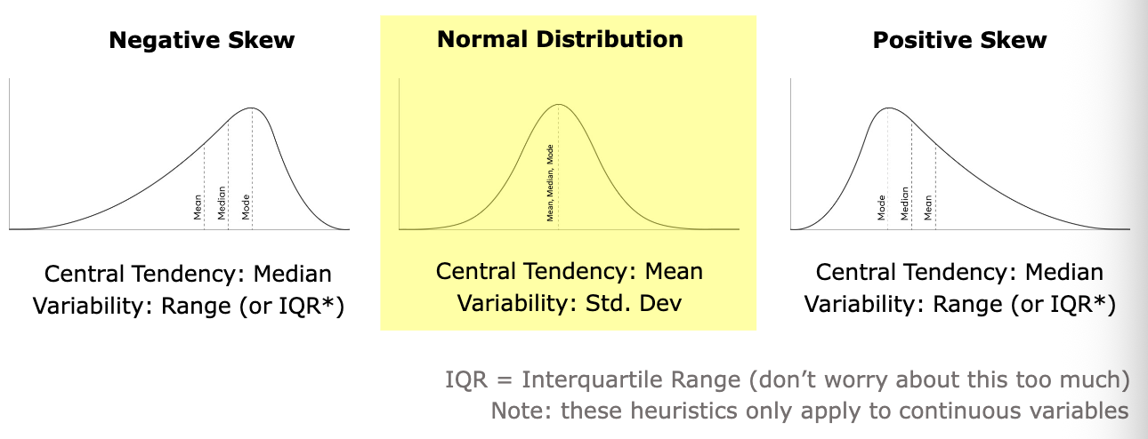
Central Tendency (center of the distribution)
e.g., mean, median, mode
Variability (spread of the distribution)
e.g., range, variance, standard deviation
Shape of the distribution
e.g., normal, positively skewed, negatively skewed
Central Tendency
Center of the distribution
Mode: most common value in the sample
Median: midpoint of the sample, sorted small → large
Mean: arithmetic average of the sample
Variability
Spread of the distribution
Range: largest value - smallest value
Variance: average of squared deviation from the mean
Find the difference (deviation) between each score and the mean
Square the deviation (get rid of the negatives)
Sum the squared deviations and divide by N - 1
Standard deviation: square root of the variance
Shape of the Distribution
Which measures of central tendency, variability should we use?
Descriptive Statistics
Short summaries to describe, interpret data sets
BDI scores were normally distributed across the sample
Point Estimation
A "point estimate” is your best guess about a single value in the population, based on your sample
Can be any value (a mean, standard deviation, a correlation…)
Simplest case is estimating the population mean
Point estimation is inferential (and inferences can be wrong, even when you do everything right)
Point Estimation: Most Important Concept
Never provide (or accept) a best guess without an associated estimate of how wrong it might be
Steps for Estimating Population Mean
Get the mean and standard deviation of your sample
Mean: arithmetic average of the sample
Standard deviation: square root of the variance
Convert to best guess and estimate of error
Best guess: population mean = sample mean
Estimate of error
Simplest version: standard error of the mean
Standard error of he mean
Want this to be small
SE will increase with sample standard deviation
SE will increase with sample size
Confidence intervals
A range of values; confident that population mean is somewhere in the range
Again, want this to be small
We typically report 95% CIs
Lower bound
Upper bound
Express in standardized/simplified format
If using standard error of the mean:
Report best guess (sample mean) ± standard error
If using 95% Confidence Interval
Report best guess (sample mean) with Ci in parentheses
Basic Components of an Experiment
At least one variable is manipulated (the assumed cause)
This is the “independent variable” (IV)
This manipulation is the defining attribute of experiments
At least one other variable is measured (the assumed effect)
This is the “dependent variable” (DV)
All other variables are controlled (the potential confounds)
Designing an Experiment
Big decision: between subjects or within-subjects?
Between- subjects: every participant experiences just one condition
e.g., 50% of participants get bright lighting; 50% get dim lighting
Within-subjects: every participants experiences all conditions
e.g., 50% of participants start with bright lighting, then move to dim lighting (and vice versa)
Each have pros + cons (validity tradeoffs)
Steps for Designing a Basic Experiment
Operationally define your variables (IV, DV)
Decide how you’ll assign participants to conditions
State your hypothesis
Internal Validity
The extent to which the observed relationship is due to causal relationships between the IV and the DV
Any threat to internal validity is a confound
Something that varies with the assumed cause (the IV)
Two potential sources of confounds (for now):
Selection effect (aka “subject confounds”)
Systematic, pre-exisiting differences between the participants in each group
Eliminate via random assignment (or matching)
Design confounds
Aspects of the conditions (not the participants) that vary with the IV
In a ‘clean’ experiment
Potential selection effects are eliminated (via random assignment/matching)
Potential design confounds are held constant (i.e., consistent across groups)
Designing an Experiment
Between-subject designs prioritize construct validity
Within-subjects designs prioritize statistical validity
Construct Validity
How well your measures assess the constructs of interest
Does your (operationally-defined) DV actually measure the construct that your care about?
A major part of construct validity depends on how you define your DV
For DVs that aren’t well-established (e.g., novel questionnaires), often useful to run preliminary studies to assess construct validity
But even with a great (validated) DV, reactivity can be a threat
Reactivity: any change in participants’ behavior due to being observed
Reactivity can be an issue in any design
Participants often want to be “good participants”
Seeing all conditions may help participants guess the hypothesis
Instead of measuring your construct, you may be measuring your participants’ beliefs about the experiment
Methods of minimizing reactivity can include:
“Hiding” your manipulation
Give participants a cover story; ask extra survey questions that you don’t care about; etc.
Talking to your participants (after the experiment)
Ask what they thought you were testing (and, if you’re really worried, exclude the ones who figured it out)
Statistical (Conclusion) Validity
How well your conclusions are justified based on your data
Are the results of my statistical tests accurate and reliable?
Did I have the statistical power to detect the effect (if it exists)?
Loosely: power is the probability of detecting a true effect; or, rejecting H0 in a world where H0 really is false
i.e., high power = lower risk of a Type II error
Individual difference can be a big threat to statistical validity
‘Noise’ that might obscure the real ‘signal’ (effect) that you care about
Individual differences can be a big issue in between-subjects designs
Back to selection effects = there may be systematic differences between groups
Minimize via random assignment, which works really well with larhe enough Ns
Functionally: need a relatively large sample to achieve high power
Individual differences are much less of an issue in within-subjects designs
The same people are in both (al) conditions!
We can account for the ‘noise’ through stats, which helps us detect the signal
Functionally: can achieve high power with a much smaller sample
Between or Within-Subjects?
Both designs prioritize internal validity (as long as you take precautions)
Watch for design confounds, selection effects (between), order effects (within)
Neither design is a great option for prioritizing high external validity
Correlational designs are a better option here
Between-subjects designs prioritize construct validity
Less risk of reactivity relative to within-subjects designs
Within-subjects designs prioritize statistical validity
High power at lower Ns
Which also makes within-subject designs more economical