True/False Review
1) Categorical data cannot be measured. Instead, data is counted and placed into a specific group or category.
2) Quantitative data is measurement data
3) Frequency looks at actual counts
4) Relative Frequency looks at data as percentages or proportions
5) Cumulative Frequency is the sum of the current count and all previous counts (a running total)
6) Cumulative Relative Frequency is the sum of the current percent and all previous percentages (a running total of the percentages or proportions)
7) A contingency table is also called a two-way table
8) If variables are dependent (not independent), then there is an association/relationship between the variables 9) If variables are independent, then there is not an association/relations between the variables 10) Pie charts and segmented bar charts should a full distribution (100%)
11) A mosaic plot is a type of segmented bar chart
12) A mosaic plot allows you to compare relative frequencies (percentages or proportions) of two or more groups
13) A mosaic plot allows you to compare the actual quantity of two more groups. Large areas have a large quantity than a smaller area.
14) Pie charts and bar charts are two ways to visually display categorical data
15) Histograms, stem-plots, and dot plots are three ways to visually display quantitative data 16) Pie charts, bar charts, histograms, stem-plots, and dot plots look at or compare one variable statistics 17) The humps on a histogram are called modes
18) The spaces on a histogram are called gaps
19) Stem-plots must have a key
20) The leaves of stem-plots are listed from least to greatest from the stems
21) When comparing two different items (ex. males vs females), you can create a back-to-back (not side-by-side) stem-plot 22) When creating a stem-plot and you have a lot of data, it is good to split the leaves from 0-4 and 5-9 23) When discussing quantitative data, you must discuss shape, center, and spread/variability 24) Never say symmetric. Instead say roughly symmetric.
25) When discussing the shape, you should discuss three things: 1) unimodal, bimodal, multimodal, or uniform 2) roughly symmetric or skewed (left/negative or right/positive), 3) gaps and outliers (if any exist)
26) Mean is the average
27) Median (Q2) is the middle number when numbers are arranged from least to greatest
28) Mode is the most occurring value
29) To find the location of the median, use the equation:
n +
1
2
30) When the sample size is odd, the median will always be the middle term
31) When the sample size is even, the median will not be a middle term, but rather the average of the two terms closest to the center
32) The mean and the median are about the same when data is roughly symmetric
33) The mean is larger than the median when data is skewed to the right (positively skewed) 34) The mean is smaller than the median when data is skewed to the left (negatively skewed) 35) The range is the maximum value minus the minimum value
36) The lower quartile (Q1) is the median of the bottom half of the data
37) The upper quartile (Q3) is the median of the top half of the data
38) The interquartile range (IQR) is Q3 – Q1
39) The range is the weakest form of variability because it is easily thrown off by outliers
40) Use the mean and standard deviation when data is roughly symmetric with no potential outliers 41) Use the median and IQR when data is skewed or outliers exist
42) The median and IQR are resistant to outliers and skewed data, but the mean and standard deviation are not resistant to outliers and skewed data
43) Standard deviation is smallest when data is tightly clustered around the mean and larger when data is more spread out (or further way from the mean)
44) The five number summary is the minimum, Q1, median, Q3, and maximum
45) The formulas for finding outliers are Q1 – 1.5(IQR) and Q3 + 1.5(IQR). These form the lower and the upper fences on boxplots.
46) Modified boxplots include outliers whereas unmodified boxplots do not include outliers
47) Unless told otherwise, always create modified boxplots
48) Whiskers should never extend to the upper and lower fences, but rather to the points just above the lower fence and just below the upper fence
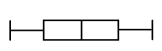
49) The boxplot below is roughly symmetric:
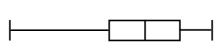
50) The boxplots below are skewed left (negatively skewed):
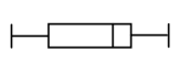
51) The boxplots below are skewed right (positively skewed):
52) Time plots are a visual displays that look at data over a period of time
53) Never extrapolate data beyond the range of the x-values
54) When adding or subtracting a value to every number in a data set (shifting data), all measures of position (mean, minimum, Q1, median, Q3, maximum) are also shifted
55) When adding or subtracting a value to every number in a data set (shifting data), all measures of spread (range, IQR, standard deviation, variance) remain the same
56) When multiplying or dividing a value to every number in a data set (rescaling data), all measures of position (mean, minimum, Q1, median, Q3, maximum) are also rescaled
57) When multiplying or dividing a value to every number in a data set (rescaling data), all measures of spread (range, IQR, standard deviation) with the exception of variance are also rescaled
58) When rescaling the variance, you must first square the value you are rescaling and then multiply/divide it by the variance
59) Population mean is
μand sample mean isx
60) Population standard deviation is
σand sample standard deviation iss
61) Population variance is2 σand sample variance is2
s
62) Percentile rank is the percentage of data that lies below an observation
63) Raw data is listing out all of the actual data
64) Summary statistics (or summary data) are statistics that summarize the data (mean, standard deviation, etc.) 65) The sample size (denoted by the letter n) is the number of observations in the sample 66) Never say that data is normal, but rather approximately normal
67) Normal models are used when histograms are unimodal and roughly symmetric 68) Normal models are used when normal probability plots are fairly linear from the lower left to the upper right 69) The center of every normal model is the mean of the data
70) Normal models are standardized when the data is converted into z-scores
71) When normal models are standardized into z-scores, the mean becomes zero
72) Z-scores have no units
73) Z-scores tell us how many standard deviations data is above or below the mean
74) When z-scores are negative, the data is below the mean. When z-scores are positive, the data is above the mean. 75) The formula for z-score is
− μ
=y
z
σ
76) Density curves look at data on or above the x-axis
77) The area of every density curve is always 1
78) The normal distribution is an example of a density curve
79) The empirical rule (68-95-99.7 rule) applies to normal models and shows that approximately 68% of data lies within 1 standard deviation of the mean, 95% of the data lies within 2 standard deviations of the mean, and 99.7% of the data lies within 3 standard deviations of the mean
80) When we have normal models and we have z-scores, we can find the probability using normalcdf
81) Normalcdf should be written as normalcdf (Lower Bound, Upper Bound,
μ , σ)
82) When you have percentages, percentile ranks, or probabilities and you want to find a z-score or critical z-statistic, then use invNorm
83) invNorm should be written invNorm (Area Below,
μ , σ)
84) Your calculator cannot find a z-score when given the top percentage of something (ie. top 5%, top 10%, etc.). You must first subtract the percentage from 100 and then use invNorm to find the z-score.
85) A trial is a sequence of events that we want to investigate that leads to an outcome
86) The law of large numbers (LLN) looks at long term behavior and says that as the number of trials increase, the repeated trials get closer and closer to the actual probability of the event
87) A simulation can be used to imitate behavior and is often used to model long term behavior 88) The following steps are used to simulate a situation:
1. Start at the beginning of a random number table and move left to right
2. Look at digits 1 at a time, 2 at a time, 3 at a time, etc. depending on the context of the question 3. Discuss how the numbers are assigned
4. Discuss if any numbers should be ignored
5. Discuss whether repeated numbers in a given trial should be ignored
6. Explain when to stop
7. Explain what to do now that the values have been selected
89) Sample Space is the collection of all possible outcomes and is denoted with the letter S
90) The result or value of the trial is called an outcome/event
91) For equally likely outcomes, every outcome in the sample space has the same probability of happening 92) Probability is always a number from 0 to 1 (0 means it will not happen, 1 means it will happen)
93) If you add all of the probabilities in a sample space, your sum will always be 1
94) The probability that the set of outcomes are not in A is called the complement of A and denotedc A. The formula is P(A ) P(A)
c= 1−
95) Disjoint events are also called Mutually Exclusive events
96) Disjoint/Mutually Exclusive events can only be one thing or the other, there can be no overlap, they cannot occur at the same time
97) The sum of all Disjoint/Mutually Exclusive events in a sample space always equals 1
98) The probability of two disjoint events happening is always 0
99) To use the Addition Rule (also called the Simple Addition Rule) events must be Disjoint/Mutually Exclusive
100) If A and B are Disjoint/Mutually Exclusive events, simply add their probability to find the probability of one or the other happening P(A U B) = P(A) + P(B)
101) Use the General Addition Rule when events are not Disjoint/Mutually Exclusive
106) Events are independent ifP A B P A ( ) = ( )
102) If A and B are not Disjoint/Mutually Exclusive events, then add their probabilities, but subtract out their intersection (if probability is denotedP A B ( )
you don’t subtract the intersection you are counting some data twice) P(A ∪ B) = P(A) + P(B) – P(A ) B) 103) It is helpful to create a Venn Diagram when events are no Disjoint/Mutually Exclusive
104) If the outcome of one event does not influence the probability of the outcome of another event, the events are said to be independent
105) Conditional probability is the probability of something happening given that something else has already happened. This .
107) Conditional probability is found using the formula
( )
P B A ∩
P A B
( )
=
P(A)
108) It is helpful to create a Tree Diagram whenever you have conditional probabilities
109) Disjoint/Mutually Exclusive events are never independent (and vice versa)
110) It is possible for events to be neither Disjoint/Mutually Exclusive nor independent
111) Drawing without replacement means that once something is drawn, that item is not put back into the pool to be selected 112) The 10% Rule for Independence is used when drawing without replacement
113) The 10% Rule for Independence says that as long as less than 10% of the population is used, you can still assume the data is independent
114) For a discrete random variable, every possible outcome can be listed
115) For a continuous random variable, there are infinite possible outcomes (thus cannot be listed). Measurements are typically continuous random variables.
116) For continuous random variables, it is helpful to standardize the data into z-scores and use a Normal Model 117) The Expected Value represents the population mean(μ)and is denoted E(X)
118) When rescaling one random variable, you do not need to work through the variance to find the standard deviation 119) When finding the standard deviation of two or more random variables, you must work through the variance 120) When subtracting two or more random variables, you add the variances
121) Bernoulli trials have exactly two possible outcomes and the events are both random and independent 122) For a Bernoulli trial, p is used to denote the probability of success and q is used to denote the probability of failure 123) Geometric models are a type of Bernoulli trial where you are looking for a first success
124) When using a graphing calculator, geometpdf(probability,trials) is used to find the probability of a first success on a given trial
125) When using a graphing calculator, geometcdf(probability,lowerbound,upperbound) is used to find the probability of a first success on or before a given trial
126) Binomial Models are used to find a specific number of successes given a specified number of Bernoulli Trials 127) The expected value and standard deviation for Binomial models are found using the following equations: E(x) = np SD(x) = npq = E(x)q
128) When using a graphing calculator, binompdf(trials, probability, successes) is used to find the probability of an exact number of successes for a given sample size
129) When using a graphing calculator, binomcdf(trials, probability,lowerbound,upperbound) is used to find the probability of a specific number of successes or fewer for a given sample size
130) The population is everyone of interest in a study
131) When you survey an entire population it is called a census
132) A sample is a smaller group within a population and should be representative (reflect the same attributes) of the population
133) A biased sample is one that over or under-represents certain characteristics of the population 134) The sampling frame is the list of the individuals for which the sample is taken
135) The sampling frame is everyone the researcher has access to. This may be the same size as the population or smaller than the population.
136) Sampling variability refers to sample to sample differences. Results from one sample to the next often differ because different individuals were chosen for each sample.
137) Pick a sampling technique based on which one does the best job of minimizing sampling variability and is representative of the population
138) You want to generalize results to the entire population (formulate conclusions that can be applied to the population). This can only happen when the sample is representative of the population.
139) The four types of random sampling techniques are simple random, stratified, cluster, and systematic 140) The two types of biased sampling techniques are convenient and volunteer (also called self-selected) 141) In simple random samples (SRS) every individual in the sampling frame has an equal chance of being selected
142) In stratified random samples, the population is divided into groups based on a common attribute before the selection of the sample takes place. Subjects are then randomly selected from each group.
143) In cluster samples, numbers are assigned to groups (rather than individuals) and groups are then randomly chosen. A census is performed on the selected groups. Each group that was assigned a number must be representative of the population.
144) In systematic samples, a system is used to select the sample (ex. every 5th person). It is good to randomly determine where to start (ex. if you randomly select a 3, then you will start with the third person and then follow your system).
145) In convenient samples, the researcher selects subjects based on who they have the easiest access
146) In volunteer (self-selected) samples, people decide for themselves whether to take part in the study (i.e. PA Systems, Megaphones, Radio/Television Commercials, Internet Advertisements, etc.). Only those with strong opinions one way or the other typically respond.
147) Valid surveys are not too long, each question asks about exactly one thing, are specific, are often quantifiable (ex. Likert Scale - strongly agree, agree, no opinion, disagree, strongly disagree), and do not include open ended questions
148) A pilot study is a trial run of a survey before giving it to a larger sample. This is also a way to identify errors and potential problems to your survey before giving it on a larger scale.
149) Nonresponse Bias - (people don’t respond to a survey) means that those who choose not to respond may have different views from those who do respond. This is the biggest issue with volunteer samples.
150) Response Bias - people do respond to a survey but their answers are influenced in some way (Wording (leading question), desire to please the researcher, not wanting to reveal/discuss things from their past or that may get them into trouble)
151) In observational studies, the researcher cannot randomly assign people groups and there are no cause and effect relationships (only associations, trends, patterns)
152) For retrospective observational studies, researchers use data that was collected in the past 153) For prospective observational studies, researchers collect data as it unfolds (or as it happens)
154) For experimental studies (comparative experimental studies), researchers randomly assign subjects to groups and researchers can make cause and effect relationships
155) Experiments are the only thing that can result in a cause and effect relationship
156) The explanatory/predictor/independent variable is what is being manipulated and the response/dependent variable is what is being measured
157) A baseline group, or a group without any treatment, is called a control group
158) Controlling sources of variability means that you want all testing conditions (besides the treatment) to be as similar as possible for every group
159) The reason we randomly assign subjects to groups is NOT to eliminate sources of variability. But rather to spread sources of variability out evenly amongst groups (equal variation amongst groups).
160) Replication means more than one individual should be in each group
161) You should block in an experiment when there is a known association (ex. Association between dog size and the amount of food dogs eat) or when something exists that is outside of the researcher’s control (ex. Land to be farmed and a river along one side of the farm land)
162) Never block based on the treatments, explanatory, or response variable
163) You should not have volunteers in a survey. However, it is okay to have volunteers in an experiment.
164) When you have volunteers in an experiment, you can only generalize your results to people with similar attributes as the volunteers.
165) If none of the subjects know which treatment they were given or the researcher doesn’t know who received the given treatments, then this is referred to as a single-blinded experiment.
166) If neither the subjects nor the researchers know how treatments were assigned, then this is referred to as a double blinded experiment.
167) A third party is typically required to blind the researchers
168) Studies involving non-humans (animals, plants, etc.) can never be double-blinded since there is no way for the non humans to know which group they are in
169) If blocking takes place, it is okay for the subjects and researcher to know how groups are blocked. So never blind based on how groups are blocked.
170) To blind the subjects, you can give them a placebo, which is something that looks just like the treatment, but isn’t the treatment (fake treatment)
171) Placebos are given to the Control Group
172) In some instances, a placebo effect takes place, which means that the people taking the placebo show some type of change
173) Whenever possible, researchers should have a control group (placebos when required) to determine whether changes take place outside of the treatment. However, sometimes it is not possible to have a control group in an experiment.
174) A lurking variable is a variable that isn’t being studied that actually does the causing. It is a variable in the background that causes something to take place.
175) Confounding variables are when you are studying multiple variables, but you don’t know which one is actually doing the causing
176) Always discuss the following when designing an experiment:
1. List all the treatments (this includes the control/placebo group if one exists)
2. Does blocking exist? If it exists, be specific on how your will block.
3. Randomization/Replication of groups/treatments. If you blocked, all treatment must be assigned in each block. 4. How will you control sources of variation?
5. Was the study blinded?
6. Explanation for what you will be measuring and comparing at the end of the study
7. Create a Diagram Whenever Possible
177) A scatterplot is a visual display when working with two quantitative variables
178) The explanatory/predictor/independent variable is along the x-axis and the response/dependent variable is along the y axis
179) The correlation coefficient (denoted r) shows the strength and direction of a linear relationship between variables.
180) The correlation coefficient has no units
181) The correlation coefficient is not impacted by shifting/rescaling/standardizing data, or swapping variables, and is sensitive to outliers.
182) The slope and correlation coefficient are always the same sign
183) The closer the correlation coefficient is to -1 or 1, the stronger the linear relationship
184) Outliers along the linear path make the correlation coefficient stronger. However, outliers off the linear path make the correlation coefficient weaker
185) A least squares regression line (linear regression line) is the line of best fit for a scatterplot
186) A residual (denoted e) is the difference between the observed and the predicted y-value
(e = observed/actual – predicted/estimated = y – yˆ)
187) A negative residual means you over-estimated your predicted y-value and a positive residual means you under estimated your predicted y-value
188) The standard deviation of the residuals is the average difference between the actual/observed and predicted/estimated y-values and has the same units as the y-values.
189) A residual plot is used to determine whether data is fairly linear. Data should look random around the x-axis (y = 0) and have no apparent patterns or trends to be fairly linear.
190) Say fairly linear/straight not linear/straight
191) The coefficient of determination (denoted2
r) is always between 0% and 100%. The closer it is to 100%, the better job
the least squares regression equation does at predicting the y-values.
192) When data (x vs y) is not fairly linear, we often re-express the data (log, square root, etc.) to make data fairly linear. Sometimes we will only re-express one of the two variables, in other cases we re-express both variables.
193) If data is re-expressed, then you know that the original data was not fairly linear prior to be re-expressed. 194)prepresents the sample proportion and p the population proportion
195) According to the Central Limit Theorem (CLT), distributions with larger samples will have smaller standard deviations (less variability) than the distributions of smaller samples
196) According to the Central Limit Theorem (CLT), the distributions of larger samples will look more normal than the distribution of smaller samples
197) The Central Limit Theorem (CLT) applies to both sampling distribution of proportions and sampling distribution of means
198) A sampling distribution of proportions uses categorical data and a sampling distribution of means using quantitative data
199) Suppose a question asks whether you should be “surprised” by the data andp = 0.35andp =0.32. When using normalcdf you should use 99 as your upper bound becausepis greater than p.
200) Suppose you roll a fair, six-sided die 500 times(n = 500). When discussing the Independence condition, you would not need to discuss the 10% rule because you are not drawing without replacement.
201) Three types of test statistics are z, t, and2 χ
202) If we are not told which confidence percentage to use, always use a 95% confidence percentage 203) If we are not told which alpha/significance level to use, always use 0.05
204) 90% confidence means that about 90% of all random samples will generate a confidence interval that contains the true proportion/mean
205) Confidence intervals always represent the middle percentage of data (ex. 95% confidence interval is the middle 95% of data)
206) For the random condition, if the question does not tell you that the sample is random, then you assume it is random
207) For the independence condition, you assume one item is independent of the next and you must discuss the 10% rule when drawing without replacement
208) When given proportions and testing the approximately normal condition, np and nq for significance tests (npandnqfor confidence intervals) must be at least 10. This is called the success/failure condition.
209) When given means and testing the approximately normal condition, the data is approximately normal if the sample size is at least 30
210) If you are trying to find the sample size and you do not know the value ofpandq, then set both equal to 0.5
211) The null hypothesis always has an equal sign, but the alternative hypothesis can have a greater than, less than, or not equal to sign
212) You have a one tailed/sided test/alternative when the alternative hypothesis has a greater than or less than sign 213) You have a two tailed/sided test/alternative when the alternative hypothesis has a not equal to sign
214) The P-value is found using normalcdf , tcdf , or2 χ cdf(depending on the type of test) and simply means to find the probability
215) If the P-value is less than or equal to an alpha level, then you will reject the null hypothesis. But, if the P-value is greater than the alpha level, then you will retain the null hypothesis.
216) The generic way of interpreting the P-value is as follows:
If we assume the null hypothesis is true, then the likelihood of getting an observed statistic at least as extreme as _________ is the P-Value.
217) For a significance test, your conclusion should have two sentences. The first should discuss the relationship between the P-value and the alpha level and whether you will retain or reject the null hypothesis. The second should link the conclusion to the context of the problem and discuss whether the evidence does not suggest (not statistically significant) or does suggest (is statistically significant) the alternative hypothesis
218) Every confidence interval should name the interval, discuss the conditions, perform the mechanics of the test (i.e. the math work), and give an interpretation of the interval
219) Every significance test should define the parameters, give the hypotheses, test the conditions, name the test, perform the mechanics of the test (i.e. the math work), and draw a conclusion
220) When the null hypothesis is outside of the confidence interval, you should reject the null hypothesis. But, when the null hypothesis is within the confidence interval, you should retain the null hypothesis.
221) A Type 1 Error occurs when you reject the null hypothesis but should have retained it 222) A Type 1 Error is often called a false positive
223) The probability of a Type 1 Error is the
α -level
224) A Type 2 Error occurs when you retain the null hypothesis but should have rejected it 225) A Type 2 Error is often called a false negative
226) The probability of a Type 2 Error is
β
227) The Power of the Test is rejecting the null hypothesis and making the correct decision to have rejected it 228) The probability of the Power of the Test is1− β
229) Lowering the
α -level makes you less likely to make a Type 1 Error, more likely to make a Type 2 Error, and decreases
the Power of the Test (because you are rejecting less often)
230) Raising the
α -level makes you more likely to make a Type 1 Error, less likely to make a Type 2 Error, and increases
the Power of the Test (because you are rejecting more often)
231) Increasing the sample size improves everything (less likely to make both a Type 1 and 2 Error and increases the Power of the Test)
232) When given one or two proportions, you always find a z-interval or conduct a z-test
233) When given means and the population standard deviation, you find a z-interval or conduct a z-test 234) When given means and the sample standard deviation you find a t-interval or conduct a t-test
235) Because you use the sample standard deviation rather than the population standard deviation for a t-interval/test, the t distribution is less normal than a normal z-distribution
236) For a 2-sample t-test, it is universally accepted to find the degrees of freedom by subtracting 1 from the smaller sample 237) For a linear regression t-test of the slope, you find the degrees of freedom by subtracting 2 from the sample size 238) tcdf should be written as tcdf (Lower Bound, Upper Bound, DF)
239) When you have percentages, percentile ranks, or probabilities and you want to find a critical t-statistic, then use invT 240) invt should be written invt (Area Below, DF)
241) When finding the sample size for a t-test, it is okay to use invNorm instead of invT to approximate the critical value 242) For a linear regression t-interval/test of the slope, you must also test the fairly linear and quantitative data condition
243) The null hypothesis for a linear regression t-test of the slope is always
β = 0 β1 = 0or
β = 0means there is no association/relationship between the two quantitative variables
244)
β≠0(two-tailed)
245) The alternative hypothesis for a linear regression t-test of the slope is almost always1 β ≠ 0or
246) When interpreting the confidence interval for a 2-proportion (sample) z-interval or a 2-sample t-interval, pay close attention to the order that you subtracted the variables and the signs (positive or negative) in your interval
248) For a 2-sample t-test, your null hypothesis is always1 2 : HO μ μ =
247) For a 2-proportion (sample) z-test, your null hypothesis is always1 2 HO: p = p 252) For a paired (matched paired) t-test, your null hypothesis is always: 0 HO μ =
249) You only pool the data when conducting a 2-proportion (sample) z-test
250) Only for a 2-proportion (sample) z-interval/test and 2-sample t-interval/test do you need to state that the groups are independent of one another.
251) Groups are not independent when conducting a paired (matched pairs) t-interval/test
253) A paired (matched paired) t-test is like a 1-sample t-test because in both cases you are running your test on a single list of data
254) A paired (matched paired) t-test is a test on the list of differences
255) You must test the paired data condition when running a paired (matched paired) t-test
256) Chi-Square tests have categorical data
257) Chi-Square models are always skewed to the right
258) Because Chi-Square models are skewed right, you never need to test the approximately normal condition 259) Chi-Square statistics are always positive
260) It is possible to have an extremely large Chi-Square Statistic.
261) For Chi-Square tests, both your null and alternative hypotheses are written as statements not equations
262) A Chi-Square Goodness of Fit Test is used when you are looking at whether the observed data (the counts) is the same as the expected counts which are found through some model/rule/theory
263) The degrees of freedom for a Chi-Square Goodness of Fit Test is categories/cells – 1
264) For Chi-Square Goodness of Fit Tests and Chi-Square Independence Tests, the conditions are random, independence (including 10% rule), counted data, and expected counts
265) For Chi-Square Homogeneity, the conditions are independence (but not 10% rule), counted data, and expected counts 266) The data for both Chi-Square Homogeneity and Chi-Square Independence Tests can be written in two-way tables 267) The process for a completing a Chi-Square Homogeneity and Chi-Square Independence Test is the same
268) If you want to determine whether multiple groups are the same, then the test is called a Chi-Square Test of Homogeneity. Key words often used for this type of test are “same,” “difference,” or “change.”
269) If you want to determine whether there is an association between the two categorical variables, then the test is called a Chi-Square Test of Independence. Key words for this type of test are “independent,” “association,” and “relationship.”
270) The Degrees of Freedom of Chi-Square Homogeneity and Chi-Square Independence Tests are found by (Rows – 1)(Columns – 1) = (R – 1)(C – 1)
271) The residual of a Chi-Square Test is found using the equation
c −
Observed Expected =
Expected
272) A negative residual for a Chi-Square Test means we observed fewer cases than we expected (we over-estimated). A positive residual for a Chi-Square Test means we observed more cases than we expected (we under-estimated).
273) If a test statistic is greater than the critical value found on a table (z, t, or chi square), then you will reject the null hypothesis.
274) If a test statistic is smaller than the critical value found on a table (z, t, or chi square), then you will retain the null hypothesis.