Visual Fields - Joanne's Revision Notes
1. Overview
Common reasons to measure fields:
Ocular signs or symptoms where perimetry assists in diagnosis
Patients who are at risk of developing a visual field defect
Congenital abnormalities associated with visual field defects
General medical history
Definitions
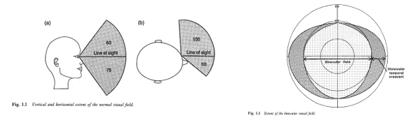
Visual field:
Portion in space in which objects are visible at same moment during steady fixation in one direction.
Monocular dimensions: 60° superiorly, 75° inferiorly, 60° nasally, 100° temporally.
Binocular dimensions: 190-200° horizontally, 60° superiorly, 75° inferiorly.
Isopter:
A line connecting points where the visual sensitivity is equal.
Kinetic Testing:
Express isopter as a fraction representing stimulus size over viewing distance.
Point of fixation:
The point at which the eye is focused during testing.
need to fixed during VF testing.
Scotoma:
An area of partial or complete loss of vision surrounded by a field of normal vision.
Absolute: doesn’t matter how bright or large, the patient can’t see it
includes the physiological blind spot.
Relative: person can’t see the target until the target is made larger or brighter.
Stimulus position, size, intensity/sensitivity:
Measured using decibels (dB).
Converted from apostilbs (asb), which aids clinical interpretation.
Standard size is size 3
Decibels (dB):
A logarithmic unit of change in brightness.
Stimulus thresholds/sensitivity (dB):
Logarithmic scale:
0 dB = maximum stimulus intensity
10 dB = intensity at 1/10 of maximum.
High dB = higher sensitivity (can detect target at lower luminance)
Higher dB indicates lower brightness needed for detection, signifying higher sensitivity.
dB not equivalent across different instruments;
Depends on background luminance and maximum stimulus luminance for that instrument.
need to use same instrument with same program and stimulus size when taking repeated measurements
Notable differences in dB values – HFA and Medmont differ by approximately ~6 dB.
Important to test patient on same instrument in serial analysis to avoid differences in dB scales
Methods of Assessing Visual Fields: Static vs. Kinetic
Kinetic Perimetry:
target is of set size and brightness
Starts in the periphery and then is brought into the centre towards the patient’s central field.
It marks the point when the px first sees the target.
Typically used in non-automated techniques.
is available on some automated projection perimeters like the Humphrey Field analyser and the Octopus (more relevant for functional analysis)
not available on the Medmont (due to set LED lights)
Advantages:
Rapid, flexible, quantifies large defects effectively.
can focus on different areas of the field (e.g., superior temporal).
Disadvantages:
Insensitive to shallow VF defects (e.g., early glaucoma).
not looking for small areas of defects → only useful for large dense defects.
Applications:
Effective for quickly locating neurological lesions
Low vision assessment
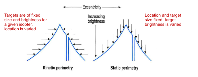
Static Perimetry
Location and target size fixed, target brightness is varied
Measured at specific locations for fixed target sizes.
usually measured using a modified staircase method.
Various strategies based on clinical needs:
Screening: measures VF using suprathreshold strategies and estimates whether the patient has a defect or not. Useful for first time patients.
Threshold: how sensitivity is affected across the field with depth of defect used for interpretation
Advantages:
quantifies sensitivity across visual field
allows detection of early VF defects
Disadvantages:
can be time consuming → fatigue effects.
faster threshold strategies use sophisticated threshold paradigms to reduce testing time without sacrificing accuracy.
Screening Techniques:
Employ rapid assessments when defects aren't anticipated.
Essential to retest using threshold techniques if any defect is initially found.
Useful to familiarise the patient with perimetric techniques prior to full threshold.
Threshold Testing Techniques:
Full Threshold:
Involves comprehensive testing to identify defects accurately.
Shorter Threshold Strategies:
e.g. SITA strategies (Standard, Fast, Faster) to efficiently identify defects.
Uses:
defect is suspected (presence of important risk factors, signs or symptoms)
patient fails screening field
baseline visual fields are required
monitoring of visual field defects required.
2. Non-Automated Methods
Confrontation:
Primarily used for detecting gross, dense visual field deficits.
Must be conducted monocularly and usually does not require correction unless in high prescription cases.
Five main methods of testing - all need to be tested on a plain background
Methods of Confrontation Testing:
Facial Amsler: Identifies central/quadrant defects using patient’s features as reference points.
Finger Counting Fields (FCF): 4 questions required to test both eyes.
Colour Comparison: Red desaturation indicates possible neurological defects.
Static Finger Movement: one finger moves in either of superior quadrants - repeated inferiorly.
Kinetic Finger Movement: finger movement or a large target to determine extent of field form non-seeing to seeing.
Amsler Chart:
Qualitative test for central visual field (~10°).
Useful for identifying central and paracentral scotomas.
also useful for areas of distorted vision close to fixation.
Advantages:
rapid
easy and portable
often used in home visits
self-monitoring
Disadvantages:
suprathreshold
relies on px to be aware of gaps / changes in fields.
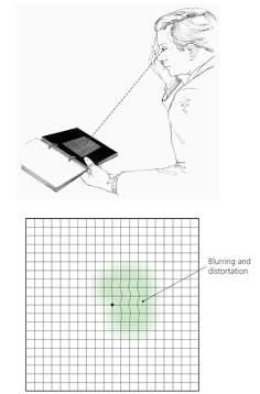
Procedure:
grid of white lines on black background
30cm working distance (need correction for someone who is presbyopic)
extends out to 10 degrees from fixation
each 5mm square subtends 1 degree.
Research:
Screening for wet AMD
useful for detecting moderate to severe glaucomatous loss
inclusion in mobile app assessments for diabetic retinopathy and AMD and telemedicine evaluations in neuro-ophthalmology.
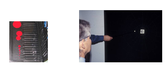
Bjerrum/Tangent Screen:
Measures central 30° at a distance of either 1 or 2 meters
uses kinetic strategy - bring wand towards centre until the px can first detect it.
Technique is flexible but examiner needs to be skilled and experienced.
consistent speed
precisely placing the pins & translating into chart.
useful in low vision.
Non-Automated Visual Field Techniques Considerations
Remember qualitative non-automated VF tests are influenced by:
Type, size, colour, brightness of targets
testing distance
speed background.
Require a skilled examiner.
qualitative visual fields tests are crude, screening tools, if any indication of abnormal results, need to perform a threshold automated test.
3. Automated Methods.
Common Automated Perimeters:
Humphrey Field Analyser (HFA):
Projected targets (based on the Goldmann bowl perimeter)
Medmont
Uses LED-targets
Other automated perimeters:
e.g., Octopus: projection systems like the HFA.
Humphrey Field Analyser Details
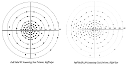
Screening tests:
can the px see the target or not? → cannot tell difference between relative or absolute defect
one zone (single intensity)
one example of a one-level screening is the Esterman test which screen at 10dB suprathreshold
included in vision standards for driver licensing in most countries.
several other screening strategies available (dependent on model) and patterns of locations
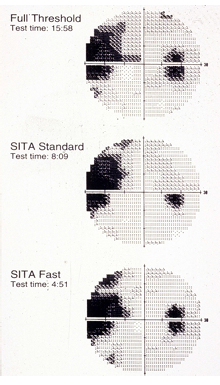
Faster Threshold Strategies:
Introduces SITA (Swedish Interactive Thresholding Algorithm) for efficient testing.
Variants:
SITA Standard: ~50% shorter than traditional methods.
SITA Fast: ~50% shorter than SITA Standard.
SITA Faster: ~30% quicker than SITA Fast.
SITA strategies reduce testing time:
detailed visual field modelling
use of information index to determine threshold endpoints
test paced to a patient’s response time
the faster the px → the faster the test.
post-test recomputation of threshold values
reduction of “catch” trials by use of inferential calculations to determine reliability.
SITA FASTER:
primary test points:
use age-corrected normal values for starting thresholds
only 1 reversal
uses field model based on SITA Fast data
retesting:
no second check for non-seen points
no false negative catch trials
fixation checked through video monitor - no blind spot checking
stimulus timing adjusted to patient responses.
Stimulus Parameters:
Sizes I-V with size III as standard
target duration set to 200ms
background illumination = 31.5 asb.
Foveal thresholds - patient fixates 4 yellow spots below fixation
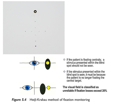
Fixation monitored using Heijl Krakau technique, corneal reflex monitoring and telescope / video.
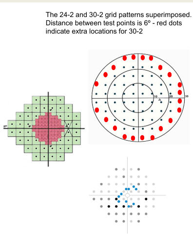
Program Patterns:
Range of programs organised on a grid
24-2 and 30-2 most commonly used: measure central 30 deg with 6 deg resolution
-1 denotes that the grid is centred on the horizontal and vertical midlines
-2 denotes a shift of 3 deg of either side of the horizontal and vertical midlines.
the -2 test grid is most commonly used
look at whether the defect crosses the meridians.
-1 and -2 grids can be merged for finer resolution
10-2 measures the central 10 deg with 2 deg resolution.
good for looking at central losses.
24-2C SITA faster adds 10 points to 24-2, to assess areas along nerve fibre bundles.
useful for early glaucoma.
custom grids also available.
Medmont Field Analyser
rear projected LED targets (target size III)
Target duration = 200ms
background luminance = 10 asb
fixation monitored by Heijl Krakau technique
Measurement strategies:
screening
threshold (bracketing 6-3) procedure
faster threshold strategies available.
Pattern of fields:
organised on an annular testing pattern
lots of different options:
e.g. Glaucoma 22 / 30 deg.
4. Factors Affecting Thresholds: Patient Factors
Age:
Kinetic perimetry shows a decrease (up to 50% between ages 20-60).
Static shows decreased sensitivity, especially superior hemifield.
Essential to use age-matched data for valid comparisons.
Pupil Size Effects:
General reduction in sensitivity - less light entering the eye.
exaggeration of defects
can dilate px pupils when doing field testing
however, will have to dilate EVERY time.
Anatomical changes
Eyelash and eyelid anatomy can obscure results
ptosis might necessitate lid taping.
be careful of corneal drying.
Prominent nose can mimic a nasal restriction.
angle px face away.
Media opacities (e.g., cataracts).
Learning Effects:
Notable learning effects seen in early exams
most evident in the superior field and beyond 30 deg (where VF sensitivity is lowest)
Fatigue:
As VF progresses short term fluctuations increase
Sensitivity may reduce with fatigue.
patients may report false negatives in established tests.
Defocus Considerations:
Correct focus is crucial for accurate perimetry
Usually results from inappropriate refractive correction for working distance of perimeter bowl.
Correct focus is best option
wide aperture lenses with no smudges / scratches
patient’s eye is centred and positioned as close to the lens as possible to avoid lens rim defects
don’t use bifocals / multifocal.
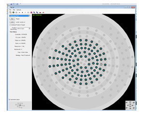
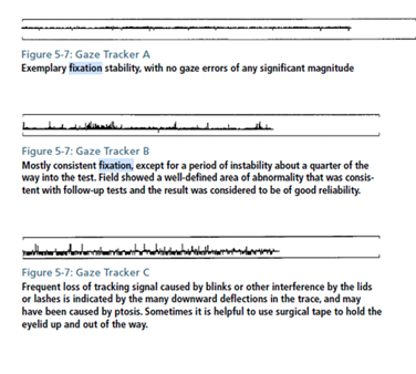
Monitoring Fixation:
Monitored by Heijl-Krakau technique as well as directly through video or telescope view of the eye and corneal reflex monitoring.
upwards lines indicate gaze errors
downward line indicates unsuccessful gaze measurement (typical blinks)
5. Factors Affecting Thresholds: Instrument Factors
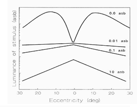
Background Luminance:
Sensitivity varies with background conditions (Weber's Law)
Most perimeters operate in photopic conditions.
shape of field changes based on rods vs cone vision
rods - gap in middle
rods & cones - flat.
Cones - peak
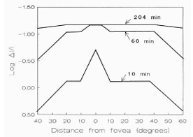
Stimulus Size Adaptation:
Small stimuli: easier to detect small defects (increased resolution)
useful for subtle defects.
large stimuli: defocus has less effect; greater dynamic range.
Stimulus Colour Input:
SWAP (Short Wavelength Automated Perimetry) utilizes a blue target against a yellow background, revealing deeper defects in glaucoma significantly earlier than traditional measures.
SITA-SWAP available: 3-6 minutes test time > 1/3 faster than standard SWAP.
SWAP:
mediated by the koniocellular pathways
compromise < 15% of cells
reduced redundancy theory
Early reports:
SWAP reveals deeper VF defects in glaucoma patients than with SAP
defects precede SAP defects by 3-5 years.
Disadvantages:
affected by lens opacities and cataracts
within and between observers variability
may be useful in diabetic retinopathy, macular oedema, neuro-ophthalmological disorders rather than glaucoma management.
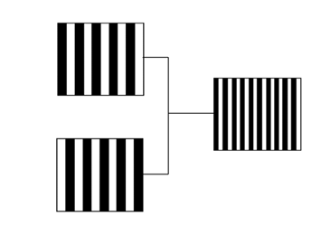
Frequency Doubling Perimetry
Focuses on isolating retinal ganglion cell subpopulations for early detection of visual field loss.
Uses the frequency doubling illusion.
FDT useful in glaucoma
BUT less reliable for neurological defects.
Mechanism:
Utilizes frequency doubling illusion through low-frequency sine gratings for detection of defects correlating with magnocellular damage in glaucoma.
Low frequency sine grating (<1 cycle per degree) flickering in counter phase at high temporal frequency (>15 Hz)
spatial frequency appears doubled - twice as many light / dark bars
believed to isolate the magnocellular M-cells that encode low-contrast, high-contrast frequency stimuli.
Evidence suggests M-cells are damaged initially in glaucoma.
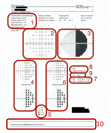
6. Visual Field Analysis
Metrics to assess validity and reliability:
1 = reliability indices
Metrics and plot to assess the type of field defect.
2 = sensitivity results (dB)
3 = Gray scale
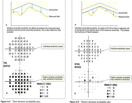
4 = Total deviation map
5 = significant values for 4 and 6
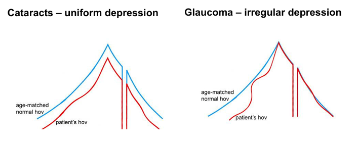
6 = pattern deviation map
7 = Mean defect (MD) and pattern standard deviation (PSD) indices
8 = Glaucoma hemifield test
9 = Visual field index
10 = gaze tracker result
Different types of plots
Gray scale plot:
darker = worse sensitivity
reasonably good overview of defect
may miss points - especially in subtle defects
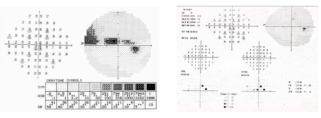
Deviation and probability plots:
total deviation = difference in px field to a normal patient.
blacker is worse = high probability of being abnormal
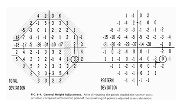
Pattern deviation map:
difference in pattern of your patient’s field compared to normal
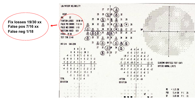
drop in sensitivity = pupil or cataract
change in shape = pattern change due to glaucoma.
highly likely to be abnormal.
Visual Field Indices
Mean sensitivity:
mean loss across the field compared to age matched normal.
Mean defect or average defect pattern standard deviation / pattern defect
A px with early glaucoma: small mean defect but big pattern defect
A px with cataract: high mean defect but small pattern defect.
pattern standard deviation / pattern defect
extent to which tested field deviates from the shape of the normal hill of vision
is a standard deviation value, so always a positive value.
Short term fluctuations:
pooled estimate of the scatter in patient responses.
the root mean variance in sensitivity
not provided in current perimeters.
Glaucoma hemifield test:
glaucoma loss tends to evade the horizontal midline.
compares upper and lower field to age matched population.
Cluster analysis:
clusters of defects.
if points are missed in different sections → less likely to be a real defect.
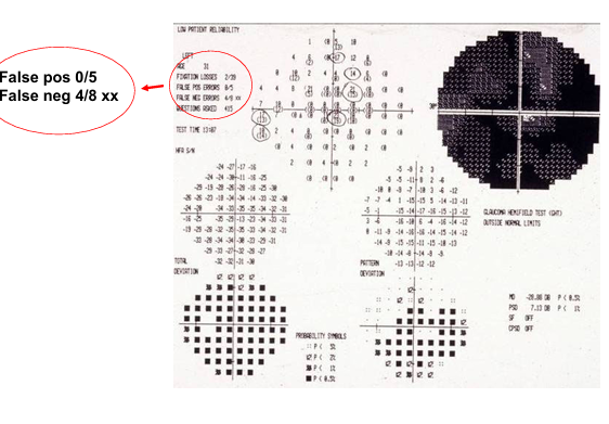
Reliability indices
3 key reliability indices used to determine whether the visual field plot is reliable:
fixation losses
false negatives
false positivies
Study of 106 random field tests in glaucoma:
fewer than two thirds of the Humphrey visual fields were considered reliable
1 in 3 tests you do is likely to be unreliable
poor reliability due to poor central fixation, inappropriate responses, poor understanding of tests
severity of visual field defects, test time and age were other factors.
visual field tests often repeated to confirm defects.
Fixation losses:
corneal reflex monitoring / Heij-Krakau method.
lots of fixation losses = unreliable.
False positive:
patient responds when there is no targeted presented (trigger happy).
px may be nervous - want to pass test.
likely to have no blind spot.
Can’t interpret the field.
False Negatives:
cloverleaf pattern
px drifts off / get sleepy
How to assess if the field is reliable?
False positive errors:
most useful of the reliability indices
15% or more suggest poor reliability → repeat test
False negative errors:
can be artificially high in glaucoma tests, particularly near edge of field defect
less critical, and while useful to assess fatigue issues not included in the newer SITA faster testing strategy
Fixation errors:
20% or more suggests poor reliability - some clinicians use a 33% rule
will be high if blind-spot not mapped correctly, even if patient demonstrates stable fixation throughout the test
may be better to rely on gaze-tracking data.
7. Serial Field Analysis
Visual field tests are inherently variable
distraction / inattentive, learning, fatigue, eye movements, other patient factors such as changes in response criteria, disease process, test administration
criteria of what is seen vs not seen.
perimetry software may contribute to test-retest variability - particular faster strategies
reduced precision in areas of reduced sensitivity and potential to mask small scotomas
test-retest reliability in areas of visual field loss can be very high ~ half the dynamic range of instrument.
High levels of disagreement between clinicians regarding whether field loss is progressing (or not), particularly in px with glaucoma.
no unified consensus on gold-standard definition of a visual field progression event and poor agreement between clinicians.
computer-assisted analysis programs have the potential to improve assessment of progression
correct the ‘noise’ and distraction of variability in data
trend-based analysis techniques developed to assess the rate of change in visual field over time
most require at least 4-5 field tests to identify progression, with more needed for trend-based data
developed for use in clinical trials and incorporated into perimetry software.
GPA (Glaucoma Progression Analysis):
Uses pattern deviation values from SITA standard or SITA fast, to correct for developing cataracts and pupil effects.
Highlights significant pointwise progression based on statistical probability using at least 3 sequential visual fields:
compares pattern deviation value to the average of 2 baseline measures
flagged if falls outside 95% test-retest variability of group of glaucoma patients classed as ‘stable’.
3 possible GPA Alerts:
No progression detected
possible progression: 3 or more test points show significant deterioration on 2 consecutive follow-up tests
Likely progression: 3 or more test points show significant deterioration on at least 3 consecutive follow-up tests
Limitations to approach:
does not predict future progression
criteria for change / progression determined from a different population of observers.
Visual Field Index
VFI is a global index (1-100%) based on an aggregate percentage of visual function
100% is a perfect age-adjusted visual field
Central visual field points are weighted more heavily
% visual field loss calculated based on pattern or total deviations depending on depth of loss.
Minimum of 5 examinations over 3 years.
VFI values plotted as a function of patient’s age to help make judgements about clinical significance of the rate of progression.
Limitations:
global change can mask pointwise changes that are typical in glaucoma
Compromise is to investigate change in pre-defined clusters
Cluster trend analysis available on Octopus
Area of ongoing research:
machine and deep learning methods
different test patterns (e.g., 10-2)
different target sizes
test frequency (e.g., frontloading)
Frontloading
involves two or more field tests on each eye in a vist
SITA-Faster Algorithm - enables multiple testing of each eye within a vist
field data from multiple tests combined to increase reliability
frontloading provides increased and earlier detection rates in glaucoma in simulation and prospective studies.
additional time and cost savings
may overcome learning or practice effects thus reducing number of visits
recent study detected twice number of glaucoma progressors at 0.5 years earlier in glaucoma.
Workflow for Visual Field Interpretation
Confirm patient and examination parameters
DOB, rx used, test pattern
Assess whether VF plot can be trusted
reliability indices, artefacts - does the test need to be repeated?
Scan across all sections
threshold values, total and pattern deviation
MD, PSD, VFI, Cluster Analysis, GPA
Describe the VF defect:
depth (shallow - deep), pattern (diffuse - localised), location.