Main Notes on Controlling Execution Plans with Hints
Notes on Controlling Execution Plans with Hints
Scope and purpose
Hints are used to influence the query optimizer’s choice of execution plan when statistics and estimates aren’t sufficient to produce the best plan. They can direct access methods, join strategies, and optimization of a set of operations for a given query.
Hints discussed here affect plan compilation and execution, not execution strategy like locking hints.
This chapter emphasizes caution: apply hints only after thorough testing and documentation; hints are not universally beneficial and can become harmful as data distributions and system versions change.
The Dangers of Using Hints
Hints are commands the optimizer must follow; if a hint is impossible to satisfy, the optimizer will still try and may throw an error (e.g., INDEX() hint).
Even when a hint seems to improve performance on one query, the same hint can degrade performance on another query or as data evolves.
Overusing hints (e.g., placing hints on most queries or procedures) indicates a root-cause problem in the workload or schema design.
Hints can remove the optimizer’s ability to adapt to data distribution changes, upgrades, or new service packs, leading to suboptimal plans over time.
The right hint on the right query can help, but the same hint on a different query or data state can cause problems like blocking and timeouts.
Hints that affect plan shape (not just execution) require careful consideration and ongoing validation.
Example risk: INDEX() hint can force a path that may be invalid for future index changes or data distribution.
Query Hints: What they control and how they are specified
Query hints take control of an entire query and can affect all operators in the execution plan.
They can force a specific operator for all aggregations, enforce a defined parameter value, or compel a new plan on every execution, or control parallelism for the query.
Syntax: the hints are specified in the OPTION clause:
SELECT … OPTION (,…);
Restrictions:
Query hints cannot be applied to data manipulation statements like INSERT (except as part of an associated SELECT).
Query hints cannot be used in subqueries because the hint must apply to the entire query.
Common hints include HASH GROUP, ORDER GROUP, MERGE UNION, HASH UNION, and various JOIN hints (LOOP, MERGE, HASH).
For more details, see Microsoft documentation (http://bit.ly/2pt7UF2).
HASH GROUP vs ORDER GROUP (Aggregation hints)
HASH GROUP: forces the query to use a Hash Match for aggregations (hash-based aggregation).
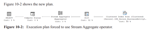
ORDER GROUP: forces the query to use a Stream Aggregate (order-based) for aggregations.
Typical scenario: A GROUP BY query with COUNT(*) may be executed with either Hash Match or Stream Aggregate depending on data characteristics.
Example scenario (Listing 10-2):
Query:
SELECT p.Suffix, COUNT(*) AS SuffixUsageCount
FROM Person.Person AS p
GROUP BY p.Suffix;
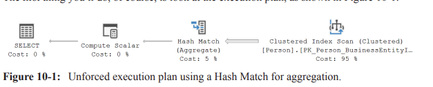
Initial plan uses Hash Match for aggregation (Hash-based). The plan shows a Hash Match (Aggregate) over a Clustered Index Scan.
Practical observation (from the example on the instructor’s system):
A non-forced Hash Match plan had measurements: ~3{,}819 reads, estimated cost 2.99727, runtime ~9.7 ext{ ms}.
Forcing ORDER GROUP (Stream Aggregate) (Listing 10-3):
SELECT p.Suffix, COUNT(*) AS SuffixUsageCount
FROM Person.Person AS p
GROUP BY p.Suffix OPTION (ORDER GROUP).
Result: the plan introduces a Sort to produce ordered input for Stream Aggregate because data must be ordered for stream aggregation.
Consequence: estimated cost increased to 4.17893, runtime ~18 ext{ ms} (about a 100% increase).
Key takeaway: forcing stream aggregation can backfire if there is no supporting index to provide ordered input, leading to expensive Sort operations.
Root-cause approach instead of hints: consider adding or modifying indexes (e.g., a nonclustered index) to enable the optimizer to use the preferred aggregation method without forcing a plan.
UNION hints: MERGE UNION, HASH UNION, CONCAT
UNION hints aim to influence how the optimizer combines results from multiple inputs.
HASH UNION: uses a Hash Match to perform the UNION operation. Note: it does not apply to UNION ALL; the optimizer will not use a Hash Match for UNION ALL concatenation.
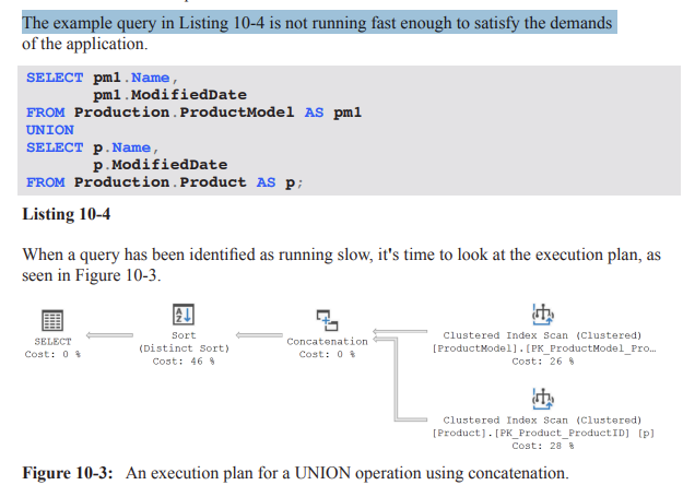
CONCAT (implicit behavior): the default behavior concatenates inputs and then removes duplicates via a Distinct Sort; this can be expensive if duplicates exist.
MERGE UNION: forces a Merge Join to implement the UNION. Merge joins require sorted inputs and can inadvertently introduce additional sorts on inputs, potentially increasing cost.
Example: UNION between Production.ProductModel and Production.Product with a MERGE UNION hint (Listing 10-5) showed that forcing a Merge Join eliminated the post-UNION Distinct Sort but added Sort operators to sort each input, raising total runtime from ~121 ext{ ms} to ~193 ext{ ms} (reads rose from 29 to 41).
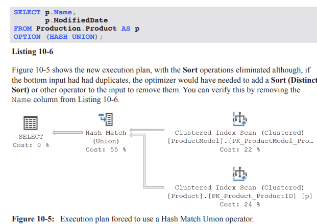
Example: applying HASH UNION (Listing 10-6) gave an execution plan with Sorts eliminated on the union output (assuming bottom input has no duplicates). Result: execution time decreased from ~121ms to ~99ms , with reads remaining around 29–41.
Practical insight: the effectiveness of UNION hints is workload- and data-dependent; a hint that helps one UNION query can hurt another, or may depend on data cardinality and duplicates.
JOIN hints: LOOP | MERGE | HASH JOIN
These hints treat all join operations in a query (including semi-joins for EXISTS/IN) using the specified join algorithm.
Important precedence rule: if you also apply a join hint on a specific join, that more granular join hint takes precedence over the general query hint.
Use case: forcing a particular join method can be useful when a particular join strategy consistently performs better for a known workload, but the risk is that changes in data distribution or schema can invalidate the assumption behind the hint.
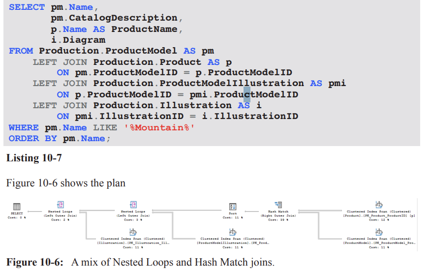
Practical example: non-SARGable predicates and mix of join strategies (Listing 10-7 and Figure 10-6)
Problem scenario: A query with a non-SARGable predicate (e.g., WHERE pm.Name LIKE '%Mountain%') prevents index seeks and leads to a Clustered Index Scan on ProductModel.
Observed plan characteristics:
The query uses a Hash Match to join Product and ProductModel, accounting for a substantial portion of estimated cost (e.g., ~39%).
A Sort operation is introduced to satisfy ordering requirements, even though the number of matching rows is estimated to be small (around 99), making the Sort relatively expensive.
The optimizer chooses to scan small, related tables rather than seek them, likely because their cost estimates are too small to elicit a different plan, resulting in nested loops for the remainder of the plan.
Takeaway: non-SARGable predicates can drive scans and hash joins; hints might not fix the underlying cost structure and can conceal the real cause (e.g., missing or unsuitable indexes).
Best practices and practical guidance
Apply hints sparingly and only after thorough testing across representative workloads and data distributions.
Document the intent, the exact hint usage, and the expected plan shape so others can understand and maintain the hint.
Schedule regular tests to verify that the hints remain valid after data changes, schema changes, or software upgrades/patches.
Always explore root causes before locking in hints: consider adding or modifying indexes, rewriting queries, or adjusting statistics rather than relying on hints for long-term stability.
Be mindful of the costs and plans that hints can introduce at runtime, including potential blocking, timeouts, or degraded concurrency if a hint prevents the optimizer from adapting to workload changes.
Remember: hints are not universal optimizers; they constrain the optimizer and can reduce future adaptability. If hints are found on many queries, re-evaluate the data model, queries, and indexing strategy.
Practical takeaways for exam readiness
Know the difference between HASH GROUP and ORDER GROUP and when each is appropriate (and the tendency for Sort operators to be introduced for ORDER GROUP).
Understand that UNION hints manipulate how UNION is executed (MERGE UNION, HASH UNION, CONCAT) and their limitations (e.g., HASH UNION with UNION ALL not applicable).
Recognize that JOIN hints (LOOP, MERGE, HASH) are global for the query but can be overridden by more granular join hints on specific join operators.
Appreciate why tests, documentation, and justification are essential when using hints; always prefer root-cause fixes (e.g., indexes) over hints when possible.
Quick reference to examples and observations mentioned in the transcript
Aggregation with HASH GROUP (default) vs ORDER GROUP (forced): cost increase due to Sort; example numbers:
Original: reads ≈ 3{,}819, estimated cost ≈ 2.99727, runtime ≈ 9.7\text{ ms}.
With ORDER GROUP: estimated cost ≈ 4.17893, runtime ≈ 18\text{ ms} (≈ 100% increase).
UNION examples:
Without hints: initial plan had a post-UNION Distinct Sort costing ~121\text{ ms} with 29 reads.
With MERGE UNION: plan avoided the post-UNION Sort but introduced sorts on inputs; runtime rose to ~193\text{ ms} with 41 reads.
With HASH UNION (assuming no duplicates on bottom input): post-union Sort eliminated; runtime improved to ~99\text{ ms} with ~29–41 reads.
Non-SARGable predicate example:
Predicate: WHERE pm.Name LIKE '%Mountain%'
Observed plan:
LOOP JOIN hint: forcing Nested Loops
Context: In experiments, forcing a specific join algorithm can change plan shape and performance. Example from the transcript: original query ran ~74\ ext{ms} with 485\ logical reads (measured via Extended Events). The LOOP JOIN hint is applied as:
Query hint: OPTION ( LOOP JOIN );
Result: optimizer is forced to use Nested Loops joins throughout the plan.
Plan changes observed:
Sorting is moved to occur directly after the scan of the ProductModel table.
Nested Loops preserves outer input order, enabling the sort to operate on about 40 rows (actual 37).
The in-memory worktable (hash/other constructs) is eliminated, as Nested Loops don’t require that worktable.
Performance observations:
Logical reads increased to 1250; runtime ~73\ ext{ms}.
Reason: Product table is scanned 37 times (once per outer row) due to the Nested Loops join, increasing I/O.
Memory considerations:
Memory grant is significantly smaller for the SELECT operator under the Nested Loops plan, which could matter for frequently executed queries.
Numerical references:
Original plan: 485\text{ logical reads}, 74\ \text{ms}.
LOOP JOIN plan: 1250\text{ logical reads}, 73\ \text{ms}.
Sort behavior: sorts about the first ~40 rows (actual 37) after the outer input.
Takeaway:
Forcing a join strategy can both reduce or increase I/O; the impact depends on data distribution, indexing, and how the plan reshapes operators (e.g., additional scans per outer input).
Evaluate memory grants and effectiveness in your workload, especially for frequently-run queries.
MERGE JOIN hint: forcing Merge Joins
Hint application: OPTION ( MERGE JOIN );
Plan shape:
The plan becomes more complex: three Sort operators appear instead of one.
Reason: Each input to the merge must be ordered on the join column; when inputs arrive unordered, extra Sorts are required.
Performance observations:
Logical reads reduced to approx. 116\text{ reads}, which is better than the LOOP JOIN option in this case.
Runtime around 83\ \text{ms} in the tests, not a performance win overall.
Trade-offs:
Overhead from the extra Sorts can offset gains from fewer reads.
Rightmost Merge Join is a many-to-many join that typically requires a worktable in tempdb, increasing memory and I/O costs (see Chapter 4, Listing 4-3 and subsequent discussion).
Takeaway:
MERGE JOIN hints can reduce reads but may incur extra sorts and worktable costs; assess with real concurrency and workload load.
HASH JOIN hint: forcing Hash Joins
Hint application: OPTION ( HASH JOIN );
Plan shape:
Three Hash Match joins, and a single Sort on the Name column (placed on the left side due to non-preservation of input order by Hash Join).
Performance observations:
Logical reads reduced to 97\text{ reads}, the best so far in the examples.
Runtime roughly similar to the original query (no clear performance improvement).
Memory considerations:
Memory grant increased significantly to about 6080\text{ KB} due to hashing all tables and building hash tables for build inputs.
Implications:
Hash joins can be beneficial when they avoid expensive lookups but can incur higher memory usage due to hashing large inputs.
If the system has memory contention, the larger memory grant may negate I/O savings.
Takeaway:
Hash Join hints can be worth testing in low-concurrency or memory-available environments, but expect higher memory pressure and potential I/O trade-offs.
The bigger problem: LIKE '%Mountain%'
Core issue:
The query uses LIKE with a leading wildcard: LIKE '%Mountain%'. This forces scans against the table and is the primary bottleneck, regardless of join hints.
Potential solutions if restructuring is possible:
Modify database structure or indexing to avoid the wildcard leading pattern.
Use computed columns, full-text search, or a search-optimized index to support the predicate efficiently.
When code or structure cannot be changed:
Query hints may yield some improvements, but they address symptoms (execution plan shape and I/O) rather than the root cause (poor predicate selectivity).
Takeaway:
Hints are often a band-aid; the most impactful long-term fix is alignment of data model and indexing with the query patterns.
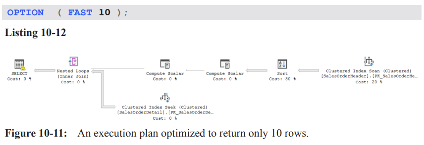
FAST n hint: returning the first n rows as fast as possible
Purpose:
The FAST n hint asks the optimizer to optimize for returning the first n rows rapidly, potentially at the expense of the rest of the result set.
Example:
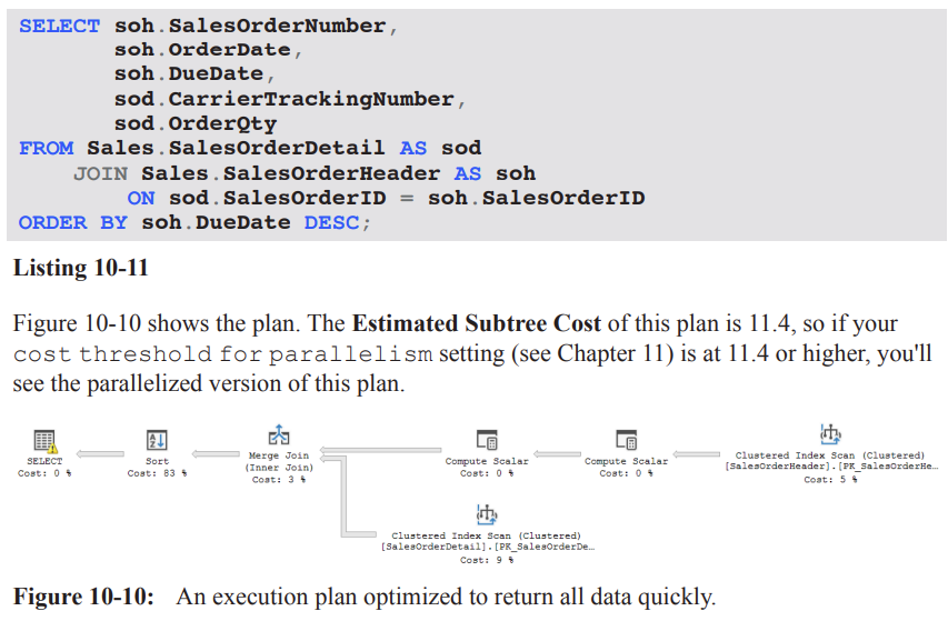
Query selects SalesOrderDetail and SalesOrderHeader joined on SalesOrderID, ordering by DueDate DESC.
Execution plan observations:
The Estimated Subtree Cost for the plan with FAST 10 is higher-level (the plan may be parallelized if the cost threshold for parallelism is exceeded, see Chapter 11).
The optimizer can choose a plan (e.g., Nested Loops) that prioritizes early row return rather than overall efficiency.
Numerical observations:
Original total estimated cost: 11.4; with FAST 10, the single-row-early plan cost becomes tuned toward the first 10 rows (example value: 2.72567 for the first 10 rows).
Note that the cost shown is for the subset of results (the first 10 rows); the actual total work remains larger.
Implications of early return:
The estimate for the first 10 rows may show favorable numbers (e.g., 2.72567) but the actual number of reads can explode when scanning the full dataset (e.g., 1{,}935 for original vs 106{,}505 with the hint in the given example).
The early-return plan often increases initial responsiveness but may degrade overall throughput and I/O efficiency when the full result set is needed.
How it works internally:
The optimizer treats the query as if it had TOP (10) and adjusts the plan accordingly by omitting operators that implement TOP while still delivering the same early results.
Takeaway:
FAST n can improve perceived responsiveness for the first n rows but can massively inflate logical reads for the full result set; balance user-perceived latency with resource usage.
FORCE ORDER hint: fix join order
Purpose:
If the optimizer’s reordering of joins is suboptimal due to outdated statistics, data skew, or complexity, you can force the query to use the join order as written.
When to consider FORCE ORDER:
Suspected that the optimizer picks a poor join order due to stale statistics or complex query with many joins.
You observe timeouts during optimization or excessive recompiles.
You have evidence that your explicit join order (as written) is better than the optimizer’s chosen order in your workload.
Example context:
A long query joins many tables (Listing 10-13) with a big, multi-table plan (Figure 10-12).
Expected effects:
The optimizer will follow the written join order rather than exploring alternative permutations.
Practical caveats:
Using FORCE ORDER can bypass potential optimizations and lead to suboptimal plans if statistics are accurate and the optimizer could have found a better order.
Testing is essential: recompile behavior, stability under load, and performance impact should be validated.
Takeaway:
FORCE ORDER is a powerful tool to control plan shape when you have high confidence in your join order; use cautiously and test thoroughly.
Large multi-table plan: optimizer timeout and early termination
Scenario:
A query with a large number of joined tables can cause optimizer timeouts due to the combinatorial explosion of join permutations.
The SELECT operator properties show a “Reason For Early Termination” due to timeout in plan generation (optimizer timeout).
Consequences:
The optimizer may not attempt all possible permutations; some potentially optimal joins may be skipped.
The resulting plan may be less than optimal for the actual data distribution.
Intervention:
If tuning via hints (e.g., FORCE ORDER) has been exhausted, you may apply hints to constrain plan shape and force a viable alternative.
Practical guidance:
Always monitor with EXPLAIN/SHOWPLAN and check the SELECT operator’s properties for timeout-related messages.
Consider indexing, statistics updates, or rewriting the query to reduce the join complexity before resorting to hints.
Key takeaways across hints and plans
Hints can shape plan choices and performance, but results are highly data- and workload-dependent:
LOOP JOIN can reduce memory pressure but may increase I/O due to repeated table scans.
MERGE JOIN can increase sorts and memory for maintaining input order, with potential gains from fewer logical reads.
HASH JOIN can minimize reads but increase memory usage due to hash tables; benefits depend on data size and available memory.
FAST n focuses on early row retrieval, boosting perceived responsiveness but potentially at the cost of overall resource use.
FORCE ORDER constrains optimizer freedom and can fix known good join orders but risks suboptimal plans if statistics are stale.
A recurring theme: the root problem in many examples is often not the join method but data filtering predicates (e.g., LIKE patterns) and data distribution.
In the provided examples, LIKE '%Mountain%' is a dominant factor driving scans and I/O; addressing the predicate or data model usually yields larger gains than hints alone.
Practical methodology:
Always measure: logical reads, memory grants, and wall-clock time (ms) across plan variants.
Compare estimated costs vs actuals; watch for misleading estimates (e.g., SORT cardinalities vs actual rows).
Consider real-world load and contention (I/O bottlenecks, memory pressure) when selecting a hint.
Use hints as a last resort after reviewing data model, indexes, and predicate selectivity; validate with representative workloads.
Notable numerical and factual references recap (with LaTeX formatting)
Original plan performance: 74\ \text{ms}, 485\text{ logical reads}.
LOOP JOIN plan: 1250\text{ logical reads}, 73\ \text{ms}; memory grant smaller.
MERGE JOIN plan: 116\text{ logical reads}, 83\ \text{ms}; memory grant nearly double; three Sort operators.
HASH JOIN plan: 97\text{ logical reads}; memory grant up to 6080\ \text{KB}; runtime similar to original.
Hint costs for FIRST N rows (FAST 10): original 11.3573 (total estimated cost) vs hinted 2.72567 (first 10 rows); actual first-row estimate vs real rows example shows 2.6 estimated vs 31465 actual rows when full execution occurs.
Forcing join order example mentioned a large multi-table plan with a timeout reason: “Reason For Early Termination” observed in the SELECT operator properties.
Parallelism threshold reference: the FAST n plan may be parallelized if its estimated subtree cost exceeds the threshold (see Chapter 11).
Practical takeaways for exam and real-world scenarios
Always start with data-model and predicate optimization (indexes, statistics, and rewriting queries) before resorting to hints.
When hints are used:
Document rationale and expected trade-offs.
Run controlled experiments with and without hints under realistic load.
Monitor memory grants, I/O, and latency to ensure the hint provides a net benefit.
Understand that hints influence the optimizer’s decisions but do not change the underlying data access costs; they can only steer execution plans.
Real-world relevance: Similar considerations apply in production systems where perceived latency (FAST n) and resource contention (memory, tempdb usage) drive tuning decisions.
Summary pointers for quick review
LOOP JOIN hint: forces Nested Loops; potential I/O increase due to multiple scans; smaller memory grants possible.
MERGE JOIN hint: can require extra Sorts; sometimes reduces reads but may increase memory and tempdb usage.
HASH JOIN hint: reduces reads but increases memory; useful under moderate memory headroom and large inputs.
FAST n hint: improves initial response; may degrade overall throughput or increase total reads; treats as TOP n for planning.
FORCE ORDER hint: locks in join order; useful when optimizer order is known to be suboptimal; requires careful testing.
Core problem often lies in predicates (e.g., LIKE with leading wildcard) rather than join strategy; structural changes may yield larger, more durable gains.
(Note: All figures, listings, and chapters referenced (e.g., Chapter 2, Listing 2-6; Chapter 4, Listing 4-3; Chapter 11) are from the same text and provide broader context for these hints and their effects.)LOOP JOIN hint: forcing Nested Loops
Context: In experiments, forcing a specific join algorithm can change plan shape and performance. Example from the transcript: original query ran ~74\ ext{ms} with 485\ logical reads (measured via Extended Events). The LOOP JOIN hint is applied as:
Query hint: OPTION ( LOOP JOIN );
Result: optimizer is forced to use Nested Loops joins throughout the plan.
Plan changes observed:
Sorting is moved to occur directly after the scan of the ProductModel table.
Nested Loops preserves outer input order, enabling the sort to operate on about 40 rows (actual 37).
The in-memory worktable (hash/other constructs) is eliminated, as Nested Loops don’t require that worktable.
Performance observations:
Logical reads increased to 1250; runtime ~73\ ext{ms}.
Reason: Product table is scanned 37 times (once per outer row) due to the Nested Loops join, increasing I/O.
Memory considerations:
Memory grant is significantly smaller for the SELECT operator under the Nested Loops plan, which could matter for frequently executed queries.
Numerical references:
Original plan: 485\text{ logical reads}, 74\ \text{ms}.
LOOP JOIN plan: 1250\text{ logical reads}, 73\ \text{ms}.
Sort behavior: sorts about the first ~40 rows (actual 37) after the outer input.
Takeaway:
Forcing a join strategy can both reduce or increase I/O; the impact depends on data distribution, indexing, and how the plan reshapes operators (e.g., additional scans per outer input).
Evaluate memory grants and effectiveness in your workload, especially for frequently-run queries.
MERGE JOIN hint: forcing Merge Joins
Hint application: OPTION ( MERGE JOIN );
Plan shape:
The plan becomes more complex: three Sort operators appear instead of one.
Reason: Each input to the merge must be ordered on the join column; when inputs arrive unordered, extra Sorts are required.
Performance observations:
Logical reads reduced to approx. 116\text{ reads}, which is better than the LOOP JOIN option in this case.
Runtime around 83\ \text{ms} in the tests, not a performance win overall.
Trade-offs:
Overhead from the extra Sorts can offset gains from fewer reads.
Rightmost Merge Join is a many-to-many join that typically requires a worktable in tempdb, increasing memory and I/O costs (see Chapter 4, Listing 4-3 and subsequent discussion).
Takeaway:
MERGE JOIN hints can reduce reads but may incur extra sorts and worktable costs; assess with real concurrency and workload load.
HASH JOIN hint: forcing Hash Joins
Hint application: OPTION ( HASH JOIN );
Plan shape:
Three Hash Match joins, and a single Sort on the Name column (placed on the left side due to non-preservation of input order by Hash Join).
Performance observations:
Logical reads reduced to 97\text{ reads}, the best so far in the examples.
Runtime roughly similar to the original query (no clear performance improvement).
Memory considerations:
Memory grant increased significantly to about 6080\text{ KB} due to hashing all tables and building hash tables for build inputs.
Implications:
Hash joins can be beneficial when they avoid expensive lookups but can incur higher memory usage due to hashing large inputs.
If the system has memory contention, the larger memory grant may negate I/O savings.
Takeaway:
Hash Join hints can be worth testing in low-concurrency or memory-available environments, but expect higher memory pressure and potential I/O trade-offs.
The bigger problem: LIKE '%Mountain%'
Core issue:
The query uses LIKE with a leading wildcard: LIKE '%Mountain%'. This forces scans against the table and is the primary bottleneck, regardless of join hints.
Potential solutions if restructuring is possible:
Modify database structure or indexing to avoid the wildcard leading pattern.
Use computed columns, full-text search, or a search-optimized index to support the predicate efficiently.
When code or structure cannot be changed:
Query hints may yield some improvements, but they address symptoms (execution plan shape and I/O) rather than the root cause (poor predicate selectivity).
Takeaway:
Hints are often a band-aid; the most impactful long-term fix is alignment of data model and indexing with the query patterns.
FAST n hint: returning the first n rows as fast as possible
Purpose:
The FAST n hint asks the optimizer to optimize for returning the first n rows rapidly, potentially at the expense of the rest of the result set.
Example:
Query selects SalesOrderDetail and SalesOrderHeader joined on SalesOrderID, ordering by DueDate DESC.
Execution plan observations:
The Estimated Subtree Cost for the plan with FAST 10 is higher-level (the plan may be parallelized if the cost threshold for parallelism is exceeded, see Chapter 11).
The optimizer can choose a plan (e.g., Nested Loops) that prioritizes early row return rather than overall efficiency.
Numerical observations:
Original total estimated cost: 11.4; with FAST 10, the single-row-early plan cost becomes tuned toward the first 10 rows (example value: 2.72567 for the first 10 rows).
Note that the cost shown is for the subset of results (the first 10 rows); the actual total work remains larger.
Implications of early return:
The estimate for the first 10 rows may show favorable numbers (e.g., 2.72567) but the actual number of reads can explode when scanning the full dataset (e.g., 1{,}935 for original vs 106{,}505 with the hint in the given example).
The early-return plan often increases initial responsiveness but may degrade overall throughput and I/O efficiency when the full result set is needed.
How it works internally:
The optimizer treats the query as if it had TOP (10) and adjusts the plan accordingly by omitting operators that implement TOP while still delivering the same early results.
Takeaway:
FAST n can improve perceived responsiveness for the first n rows but can massively inflate logical reads for the full result set; balance user-perceived latency with resource usage.
FORCE ORDER hint: fix join order
Purpose:
If the optimizer’s reordering of joins is suboptimal due to outdated statistics, data skew, or complexity, you can force the query to use the join order as written.
When to consider FORCE ORDER:
Suspected that the optimizer picks a poor join order due to stale statistics or complex query with many joins.
You observe timeouts during optimization or excessive recompiles.
You have evidence that your explicit join order (as written) is better than the optimizer’s chosen order in your workload.
Example context:
A long query joins many tables (Listing 10-13) with a big, multi-table plan (Figure 10-12).
Expected effects:
The optimizer will follow the written join order rather than exploring alternative permutations.
Practical caveats:
Using FORCE ORDER can bypass potential optimizations and lead to suboptimal plans if statistics are accurate and the optimizer could have found a better order.
Testing is essential: recompile behavior, stability under load, and performance impact should be validated.
Takeaway:
FORCE ORDER is a powerful tool to control plan shape when you have high confidence in your join order; use cautiously and test thoroughly.
Large multi-table plan: optimizer timeout and early termination
Scenario:
A query with a large number of joined tables can cause optimizer timeouts due to the combinatorial explosion of join permutations.
The SELECT operator properties show a “Reason For Early Termination” due to timeout in plan generation (optimizer timeout).
Consequences:
The optimizer may not attempt all possible permutations; some potentially optimal joins may be skipped.
The resulting plan may be less than optimal for the actual data distribution.
Intervention:
If tuning via hints (e.g., FORCE ORDER) has been exhausted, you may apply hints to constrain plan shape and force a viable alternative.
Practical guidance:
Always monitor with EXPLAIN/SHOWPLAN and check the SELECT operator’s properties for timeout-related messages.
Consider indexing, statistics updates, or rewriting the query to reduce the join complexity before resorting to hints.
Key takeaways across hints and plans
Hints can shape plan choices and performance, but results are highly data- and workload-dependent:
LOOP JOIN can reduce memory pressure but may increase I/O due to repeated table scans.
MERGE JOIN can increase sorts and memory for maintaining input order, with potential gains from fewer logical reads.
HASH JOIN can minimize reads but increase memory usage due to hash tables; benefits depend on data size and available memory.
FAST n focuses on early row retrieval, boosting perceived responsiveness but potentially at the cost of overall resource use.
FORCE ORDER constrains optimizer freedom and can fix known good join orders but risks suboptimal plans if statistics are stale.
A recurring theme: the root problem in many examples is often not the join method but data filtering predicates (e.g., LIKE patterns) and data distribution.
In the provided examples, LIKE '%Mountain%' is a dominant factor driving scans and I/O; addressing the predicate or data model usually yields larger gains than hints alone.
Practical methodology:
Always measure: logical reads, memory grants, and wall-clock time (ms) across plan variants.
Compare estimated costs vs actuals; watch for misleading estimates (e.g., SORT cardinalities vs actual rows).
Consider real-world load and contention (I/O bottlenecks, memory pressure) when selecting a hint.
Use hints as a last resort after reviewing data model, indexes, and predicate selectivity; validate with representative workloads.
Notable numerical and factual references recap (with LaTeX formatting)
Original plan performance: 74\ \text{ms}, 485\text{ logical reads}.
LOOP JOIN plan: 1250\text{ logical reads}, 73\ \text{ms}; memory grant smaller.
MERGE JOIN plan: 116\text{ logical reads}, 83\ \text{ms}; memory grant nearly double; three Sort operators.
HASH JOIN plan: 97\text{ logical reads}; memory grant up to 6080\ \text{KB}; runtime similar to original.
Hint costs for FIRST N rows (FAST 10): original 11.3573 (total estimated cost) vs hinted 2.72567 (first 10 rows); actual first-row estimate vs real rows example shows 2.6 estimated vs 31465 actual rows when full execution occurs.
Forcing join order example mentioned a large multi-table plan with a timeout reason: “Reason For Early Termination” observed in the SELECT operator properties.
Parallelism threshold reference: the FAST n plan may be parallelized if its estimated subtree cost exceeds the threshold (see Chapter 11).
Practical takeaways for exam and real-world scenarios
Always start with data-model and predicate optimization (indexes, statistics, and rewriting queries) before resorting to hints.
When hints are used:
Document rationale and expected trade-offs.
Run controlled experiments with and without hints under realistic load.
Monitor memory grants, I/O, and latency to ensure the hint provides a net benefit.
Understand that hints influence the optimizer’s decisions but do not change the underlying data access costs; they can only steer execution plans.
Real-world relevance: Similar considerations apply in production systems where perceived latency (FAST n) and resource contention (memory, tempdb usage) drive tuning decisions.
Summary pointers for quick review
LOOP JOIN hint: forces Nested Loops; potential I/O increase due to multiple scans; smaller memory grants possible.
MERGE JOIN hint: can require extra Sorts; sometimes reduces reads but may increase memory and tempdb usage.
HASH JOIN hint: reduces reads but increases memory; useful under moderate memory headroom and large inputs.
FAST n hint: improves initial response; may degrade overall throughput or increase total reads; treats as TOP n for planning.
FORCE ORDER hint: locks in join order; useful when optimizer order is known to be suboptimal; requires careful testing.
Core problem often lies in predicates (e.g., LIKE with leading wildcard) rather than join strategy; structural changes may yield larger, more durable gains.
(Note: All figures, listings, and chapters referenced (e.g., Chapter 2, Listing 2-6; Chapter 4, Listing 4-3; Chapter 11) are from the same text and provide broader context for these hints and their effects.)Hash Join with a significant portion of cost; a Sort was introduced to enforce order; scans chosen for small tables due to cost estimates.
External references and further reading
For deeper details on hints, consult Microsoft docs at the provided link: http://bit.ly/2pt7UF2
The discussion emphasizes that hints are a tool of last resort and should be used with caution and robust testing.
Summary
Hints can guide the optimizer to a better plan in some situations, but they also reduce adaptability and can become harmful as data evolves.
The safest path is to diagnose root causes (statistics, indexes, query structure) and use hints only when tested, documented, and clearly justified.
Always balance short-term gains against long-term maintainability and plan stability.
LOOP JOIN hint: forcing Nested Loops
Context: In experiments, forcing a specific join algorithm can change plan shape and performance. Example from the transcript: original query ran ~74\ ext{ms} with 485\ logical reads (measured via Extended Events). The LOOP JOIN hint is applied as:
Query hint: OPTION ( LOOP JOIN );
Result: optimizer is forced to use Nested Loops joins throughout the plan.
Plan changes observed:
Sorting is moved to occur directly after the scan of the ProductModel table.
Nested Loops preserves outer input order, enabling the sort to operate on about 40 rows (actual 37).
The in-memory worktable (hash/other constructs) is eliminated, as Nested Loops don’t require that worktable.
Performance observations:
Logical reads increased to 1250; runtime ~73\ ext{ms}.
Reason: Product table is scanned 37 times (once per outer row) due to the Nested Loops join, increasing I/O.
Memory considerations:
Memory grant is significantly smaller for the SELECT operator under the Nested Loops plan, which could matter for frequently executed queries.
Numerical references:
Original plan: 485\text{ logical reads}, 74\ \text{ms}.
LOOP JOIN plan: 1250\text{ logical reads}, 73\ \text{ms}.
Sort behavior: sorts about the first ~40 rows (actual 37) after the outer input.
Takeaway:
Forcing a join strategy can both reduce or increase I/O; the impact depends on data distribution, indexing, and how the plan reshapes operators (e.g., additional scans per outer input).
Evaluate memory grants and effectiveness in your workload, especially for frequently-run queries.
MERGE JOIN hint: forcing Merge Joins
Hint application: OPTION ( MERGE JOIN );
Plan shape:
The plan becomes more complex: three Sort operators appear instead of one.
Reason: Each input to the merge must be ordered on the join column; when inputs arrive unordered, extra Sorts are required.
Performance observations:
Logical reads reduced to approx. 116\text{ reads}, which is better than the LOOP JOIN option in this case.
Runtime around 83\ \text{ms} in the tests, not a performance win overall.
Trade-offs:
Overhead from the extra Sorts can offset gains from fewer reads.
Rightmost Merge Join is a many-to-many join that typically requires a worktable in tempdb, increasing memory and I/O costs (see Chapter 4, Listing 4-3 and subsequent discussion).
Takeaway:
MERGE JOIN hints can reduce reads but may incur extra sorts and worktable costs; assess with real concurrency and workload load.
HASH JOIN hint: forcing Hash Joins
Hint application: OPTION ( HASH JOIN );
Plan shape:
Three Hash Match joins, and a single Sort on the Name column (placed on the left side due to non-preservation of input order by Hash Join).
Performance observations:
Logical reads reduced to 97\text{ reads}, the best so far in the examples.
Runtime roughly similar to the original query (no clear performance improvement).
Memory considerations:
Memory grant increased significantly to about 6080\text{ KB} due to hashing all tables and building hash tables for build inputs.
Implications:
Hash joins can be beneficial when they avoid expensive lookups but can incur higher memory usage due to hashing large inputs.
If the system has memory contention, the larger memory grant may negate I/O savings.
Takeaway:
Hash Join hints can be worth testing in low-concurrency or memory-available environments, but expect higher memory pressure and potential I/O trade-offs.
The bigger problem: LIKE '%Mountain%'
Core issue:
The query uses LIKE with a leading wildcard: LIKE '%Mountain%'. This forces scans against the table and is the primary bottleneck, regardless of join hints.
Potential solutions if restructuring is possible:
Modify database structure or indexing to avoid the wildcard leading pattern.
Use computed columns, full-text search, or a search-optimized index to support the predicate efficiently.
When code or structure cannot be changed:
Query hints may yield some improvements, but they address symptoms (execution plan shape and I/O) rather than the root cause (poor predicate selectivity).
Takeaway:
Hints are often a band-aid; the most impactful long-term fix is alignment of data model and indexing with the query patterns.
FAST n hint: returning the first n rows as fast as possible
Purpose:
The FAST n hint asks the optimizer to optimize for returning the first n rows rapidly, potentially at the expense of the rest of the result set.
Example:
Query selects SalesOrderDetail and SalesOrderHeader joined on SalesOrderID, ordering by DueDate DESC.
Execution plan observations:
The Estimated Subtree Cost for the plan with FAST 10 is higher-level (the plan may be parallelized if the cost threshold for parallelism is exceeded, see Chapter 11).
The optimizer can choose a plan (e.g., Nested Loops) that prioritizes early row return rather than overall efficiency.
Numerical observations:
Original total estimated cost: 11.4; with FAST 10, the single-row-early plan cost becomes tuned toward the first 10 rows (example value: 2.72567 for the first 10 rows).
Note that the cost shown is for the subset of results (the first 10 rows); the actual total work remains larger.
Implications of early return:
The estimate for the first 10 rows may show favorable numbers (e.g., 2.72567) but the actual number of reads can explode when scanning the full dataset (e.g., 1{,}935 for original vs 106{,}505 with the hint in the given example).
The early-return plan often increases initial responsiveness but may degrade overall throughput and I/O efficiency when the full result set is needed.
How it works internally:
The optimizer treats the query as if it had TOP (10) and adjusts the plan accordingly by omitting operators that implement TOP while still delivering the same early results.
Takeaway:
FAST n can improve perceived responsiveness for the first n rows but can massively inflate logical reads for the full result set; balance user-perceived latency with resource usage.
FORCE ORDER hint: fix join order
Purpose:
If the optimizer’s reordering of joins is suboptimal due to outdated statistics, data skew, or complexity, you can force the query to use the join order as written.
When to consider FORCE ORDER:
Suspected that the optimizer picks a poor join order due to stale statistics or complex query with many joins.
You observe timeouts during optimization or excessive recompiles.
You have evidence that your explicit join order (as written) is better than the optimizer’s chosen order in your workload.
Example context:
A long query joins many tables (Listing 10-13) with a big, multi-table plan (Figure 10-12).
Expected effects:
The optimizer will follow the written join order rather than exploring alternative permutations.
Practical caveats:
Using FORCE ORDER can bypass potential optimizations and lead to suboptimal plans if statistics are accurate and the optimizer could have found a better order.
Testing is essential: recompile behavior, stability under load, and performance impact should be validated.
Takeaway:
FORCE ORDER is a powerful tool to control plan shape when you have high confidence in your join order; use cautiously and test thoroughly.
Large multi-table plan: optimizer timeout and early termination
Scenario:
A query with a large number of joined tables can cause optimizer timeouts due to the combinatorial explosion of join permutations.
The SELECT operator properties show a “Reason For Early Termination” due to timeout in plan generation (optimizer timeout).
Consequences:
The optimizer may not attempt all possible permutations; some potentially optimal joins may be skipped.
The resulting plan may be less than optimal for the actual data distribution.
Intervention:
If tuning via hints (e.g., FORCE ORDER) has been exhausted, you may apply hints to constrain plan shape and force a viable alternative.
Practical guidance:
Always monitor with EXPLAIN/SHOWPLAN and check the SELECT operator’s properties for timeout-related messages.
Consider indexing, statistics updates, or rewriting the query to reduce the join complexity before resorting to hints.
Key takeaways across hints and plans - REVIEW HERE
Hints can shape plan choices and performance, but results are highly data- and workload-dependent:
LOOP JOIN can reduce memory pressure but may increase I/O due to repeated table scans.
MERGE JOIN can increase sorts and memory for maintaining input order, with potential gains from fewer logical reads.
HASH JOIN can minimize reads but increase memory usage due to hash tables; benefits depend on data size and available memory.
FAST n focuses on early row retrieval, boosting perceived responsiveness but potentially at the cost of overall resource use.
FORCE ORDER constrains optimizer freedom and can fix known good join orders but risks suboptimal plans if statistics are stale.
A recurring theme: the root problem in many examples is often not the join method but data filtering predicates (e.g., LIKE patterns) and data distribution.
In the provided examples, LIKE '%Mountain%' is a dominant factor driving scans and I/O; addressing the predicate or data model usually yields larger gains than hints alone.
Practical methodology:
Always measure: logical reads, memory grants, and wall-clock time (ms) across plan variants.
Compare estimated costs vs actuals; watch for misleading estimates (e.g., SORT cardinalities vs actual rows).
Consider real-world load and contention (I/O bottlenecks, memory pressure) when selecting a hint.
Use hints as a last resort after reviewing data model, indexes, and predicate selectivity; validate with representative workloads.
Notable numerical and factual references recap (with LaTeX formatting)
Original plan performance: 74\ \text{ms}, 485\text{ logical reads}.
LOOP JOIN plan: 1250\text{ logical reads}, 73\ \text{ms}; memory grant smaller.
MERGE JOIN plan: 116\text{ logical reads}, 83\ \text{ms}; memory grant nearly double; three Sort operators.
HASH JOIN plan: 97\text{ logical reads}; memory grant up to 6080\ \text{KB}; runtime similar to original.
Hint costs for FIRST N rows (FAST 10): original 11.3573 (total estimated cost) vs hinted 2.72567 (first 10 rows); actual first-row estimate vs real rows example shows 2.6 estimated vs 31465 actual rows when full execution occurs.
Forcing join order example mentioned a large multi-table plan with a timeout reason: “Reason For Early Termination” observed in the SELECT operator properties.
Parallelism threshold reference: the FAST n plan may be parallelized if its estimated subtree cost exceeds the threshold (see Chapter 11).
Practical takeaways for exam and real-world scenarios
Always start with data-model and predicate optimization (indexes, statistics, and rewriting queries) before resorting to hints.
When hints are used:
Document rationale and expected trade-offs.
Run controlled experiments with and without hints under realistic load.
Monitor memory grants, I/O, and latency to ensure the hint provides a net benefit.
Understand that hints influence the optimizer’s decisions but do not change the underlying data access costs; they can only steer execution plans.
Real-world relevance: Similar considerations apply in production systems where perceived latency (FAST n) and resource contention (memory, tempdb usage) drive tuning decisions.
Summary pointers for quick review (P2)
LOOP JOIN hint: forces Nested Loops; potential I/O increase due to multiple scans; smaller memory grants possible.
MERGE JOIN hint: can require extra Sorts; sometimes reduces reads but may increase memory and tempdb usage.
HASH JOIN hint: reduces reads but increases memory; useful under moderate memory headroom and large inputs.
FAST n hint: improves initial response; may degrade overall throughput or increase total reads; treats as TOP n for planning.
FORCE ORDER hint: locks in join order; useful when optimizer order is known to be suboptimal; requires careful testing.
Core problem often lies in predicates (e.g., LIKE with leading wildcard) rather than join strategy; structural changes may yield larger, more durable gains.
(Note: All figures, listings, and chapters referenced (e.g., Chapter 2, Listing 2-6; Chapter 4, Listing 4-3; Chapter 11) are from the same text and provide broader context for these hints and their effects.)
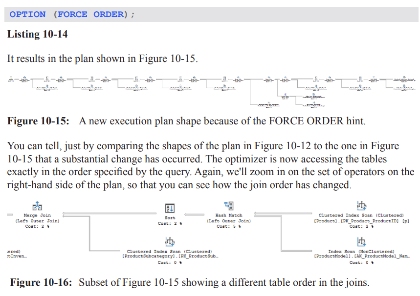
FORCE ORDER
OPTION (FORCE ORDER) can drastically change the execution plan shape by forcing the optimizer to access the tables in the exact order specified by the query. This is visible when comparing Plan shapes (Figures 10-12 vs 10-15 in the material).
In the example, the join order becomes: Product → ProductModel → ProductSub-Category → ProductInventory → … (as described in the text). This new order feeds into a Merge Join pipeline.
The left side of the plan shows a different subset of operators after forcing the order; specifically, the top input to a Merge Join to ProductSub-Category becomes the Product table first, then ProductModel, etc. This can cause more Sort operations to be needed.
Result: execution time increased from 149\text{ ms} to 166\text{ ms} in the example, demonstrating that forcing a particular join order does not guarantee better performance.
Takeaway: Direct control over the optimizer via hints can yield worse results; use FORCE ORDER with caution and validate performance impacts across representative workloads.
MAXDOP and parallelism control
Two contrasting plans for a given query were observed: a serial plan that runs quickly (Figure 10-17) and a parallel plan (Figure 10-18) that, in this case, runs slower.
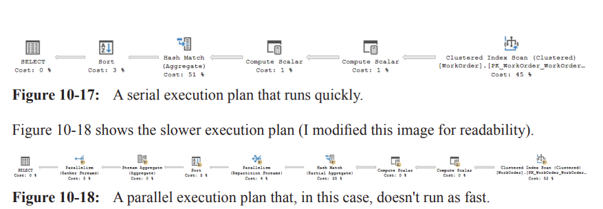
Why parallelism occurred:
The optimizer estimated that the serial cost might exceed the 'cost threshold for parallelism' (the server-side threshold controlled by cost\ threshold\ for\ parallelism).
This led to the creation of a parallel plan that distributes work across multiple CPUs (discussed in Chapter 11).
Practical implication: parallelism is not always beneficial; improper conditions can make it slower due to overheads from splitting data streams and aggregating results.
How to address:
Per-server configuration: set MAXDOP at the server level to control maximum degree of parallelism across queries.
Per-database configuration: often a better approach than server-wide settings.
Tune the cost\ threshold\ for\ parallelism so only truly high-cost queries use parallelism. A common recommendation is not to leave the threshold at the default of 5; see the referenced blog post for details.
Per-query control: use the MAXDOP hint to govern parallelism for individual queries instead of changing server-wide settings.
Example of MAXDOP control:
To suppress parallelism for a particular query, use Option(MAXDOP 1). The plan becomes serial (no parallel workers).
More commonly, set a MAXDOP value greater than 1 but less than the number of processors to limit resource hogging while still permitting some parallelism.
Summary: Per-query MAXDOP gives you finer control than server-level settings and helps prevent long-running queries from monopolizing CPUs. However, the usefulness of parallelism depends on the specific workload and data distribution.
Practical note: after experimenting with parallelism, you may temporarily lower the threshold (e.g., to force parallelism for demonstration) and then revert to normal values (e.g., EXEC sys.sp_configure \ 'cost threshold for parallelism\', 5; ) to restore default behavior.
The example also shows how to enable advanced options temporarily to adjust the cost threshold, and then revert with RECONFIGURE WITH OVERRIDE.
OPTIMIZE FOR and parameter sniffing
Problem context: Parameter sniffing can cause a parameterized query to pick a plan that performs well for some parameter values but poorly for others.
Hint solution: OPTIMIZE FOR instructs the optimizer to optimize for a specific parameter value (or an UNKNOWN value) rather than sniffed values from the first execution.
With SQL Server 2008 and later, you can use OPTIMIZE FOR with a concrete value or with a value of UNKNOWN to force a more generic plan.
Example scenario (Mentor vs London):
Two simple queries return data from Person.Address with a WHERE clause on City given different values.
Queries:
Mentor: City = 'Mentor'
London: City = 'London'
Both queries are run together, producing two different execution plans (Figure 10-19).
Mentor plan details: scans Address to locate matches, then a Key Lookup to retrieve rest of the data, joined via Nested Loops.
London plan details: due to lower selectivity, a scan of the clustered index is chosen instead, not a Key Lookup.
Reuse caveat: If this were inside a stored procedure, the plan that was compiled first for, say, Mentor might be reused for London in subsequent executions, leading to poor performance for the second value.
OPTIMIZE FOR (@City = 'London') can be used to tailor a plan to a specific value, but it risks becoming “bad” as data changes (data distribution shifts over time).
A safer general strategy is OPTIMIZE FOR UNKNOWN, which yields a more generic plan based on density estimates and average distributions, avoiding sniffed values.
Local variables impact sniffing:
Using local variables in T‑SQL (e.g., DECLARE @City NVARCHAR(30); SET @City = 'Mentor'; …) prevents the optimizer from sniffing the actual value at compile time (unless a statement-level RECOMPILE happens via OPTION (RECOMPILE)).
In this case, the optimizer uses the density value to estimate cardinality, producing plans that often look the same for different input values.
In Listing 10-18, City = @City yields identical plans for Mentor and London because the optimizer cannot sniff the actual value.
Implication: To force a generic plan for queries with variables, consider OPTIMIZE FOR UNKNOWN or use RECOMPILE strategically (covered later) to sniff values when appropriate.
Practical guidance:
Avoid relying on OPTIMIZE FOR when data distributions change or when the workload is unpredictable.
Use OPTIMIZE FOR UNKNOWN to obtain a robust, generic plan when you want to avoid sniffing pitfalls.
If a particular value is known to be problematic, you might experiment with OPTIMIZE FOR (@City = 'London') for targeted optimization, but monitor for data-change effects.
Quick recap: parameter sniffing can cause plan instability; OPTIMIZE FOR and UNKNOWN provide mechanisms to stabilize plans, but they come with tradeoffs in adaptability as data evolves.
Local variables, recompile hints, and plan stability
Local variables prevent the optimizer from sniffing actual values during compilation (unless an OPTION (RECOMPILE) is used).
Consequently, the optimizer bases cardinality estimates on density and average distributions, which can yield suboptimal plans for specific parameter values.
When the exact value matters, you can use OPTION (RECOMPILE) to trigger a statement-level recompile so the optimizer can sniff the actual value on each execution.
The material points to future discussion of RECOMPILE and related hints, indicating that these tools provide more granular control over when recompilation occurs.
Practical implications and best practices
Use hints like FORCE ORDER, MAXDOP, and OPTIMIZE FOR sparingly. Hints can fix problems but can also hurt performance if the underlying data distribution or workload changes.
Favor server-wide and database-wide configuration when possible (e.g., adjusting MAXDOP and cost\ threshold\ for\ parallelism) before relying on per-query hints.
Use Extended Events or Query Store to monitor plan changes over time and across parameter variations to identify when hints are beneficial or harmful.
For parameter sniffing issues, OPTIMIZE FOR UNKNOWN is often a safer default than pinning to a specific value.
If a specific value must be optimized for, consider testing both a targeted OPTIMIZE FOR and a more generic approach, and watch for data skew as data evolves.
Always compare execution plans and actual runtimes for representative workloads when applying hints or making configuration changes.
Notable references and follow-ups
The material notes that tuning the cost threshold for parallelism is discussed in detail in a related blog post (link provided in the text).
Chapter 8 discusses parameter sniffing in depth and introduces concepts around sniffed vs generic plans.
Chapter 11 provides more detail on parallelism internals and how the optimizer assigns costs across CPUs.
The examples reference multiple figures (Figures 10-17, 10-18, 10-19) and listings (Listings 10-15 through 10-19) that illustrate serial vs parallel plans, and parameter sniffing scenarios.
The OPTIMIZE FOR UNKNOWN approach is highlighted as a practical way to stabilize plans in the face of changing data distributions.
Quick reference: key terms and parameters
FORCE ORDER: Hints the optimizer to follow the user-specified join order.
MAXDOP: Maximum Degree Of Parallelism; per-query control to limit parallel workers.
cost threshold for parallelism: Server-level threshold that determines when to use a parallel plan.
OPTIMIZE FOR: Hint to tailor optimization for a particular parameter value or UNKNOWN for a generic plan.
UNKNOWN: A value used with OPTIMIZE FOR to force a generic plan, avoiding sniffed values.
parameter sniffing: The phenomenon where the optimizer creates a plan optimized for the first parameter values seen, which may not be optimal for subsequent values.
RECOMPILE: Hint that forces a recompile for a query, enabling sniffing of actual parameter values on each execution.
Local variables: Variables declared in T‑SQL; using them can prevent sniffing and lead to generic plans unless RECOMPILE is used.
Key Lookup, Nested Loops, Merge Join, Sort: Examples of operators that can appear in plans and are sensitive to join order and parallelism.
Summary takeaways (P3)
Hints can dramatically alter execution plans and performance; use them judiciously and validate with representative workloads.
Parallelism can help or hurt; tuning MAXDOP and the cost\ threshold\ for\ parallelism thoughtfully is usually more robust than forcing per-query parallelism.
Parameter sniffing can cause performance variability across parameter values; strategies include OPTIMIZE FOR UNKNOWN, OPTIMIZE FOR with specific values, and occasional RECOMPILE.
Local variables help prevent sniffing but may lead to suboptimal plans unless you recompile or otherwise tailor the plan.
Use monitoring (Extended Events, Query Store) to observe how plans change over time and under different parameter values to guide hint usage and configuration choices.
OPTIMIZE FOR UNKNOWN
Context: Used in a procedure to influence the execution plan for a predicate that might be highly selective or uncommon.
Example snippet (from Listing 10-19):
  CREATE OR ALTER PROCEDURE dbo.AddressByCity
    @City NVARCHAR(30) AS
  SELECT AddressID, AddressLine1, AddressLine2, City, StateProvinceID, PostalCode, SpatialLocation, rowguid, ModifiedDate
  FROM  Person.Address
  WHERE City = @City
  OPTION (OPTIMIZE FOR UNKNOWN);
  GO
  EXEC dbo.AddressByCity @City = N'Mentor';
Effect observed:
Even though Mentor is an uncommon city and the index is selective for the predicate, the plan produced is the generic plan rather than one tailored to a specific city value.
Practical takeaway:
OPTIMIZE FOR UNKNOWN is a powerful hint but requires intimate knowledge of the data distribution and query workload.
Choosing the wrong value for OPTIMIZE FOR can hurt performance.
You should maintain and re-evaluate the hint as data changes over time.
Extending to multiple variables:
If you need to control optimization for more than one variable, you can specify multiple hints in the OPTIMIZE FOR clause.
Example (as per Listing 10-20):
OPTION (OPTIMIZE FOR (@City = 'London', @PostalCode = 'W1Y 3RA'))OPTIMIZE FOR (specific values) and guidance
Listing 10-20 demonstrates how to target optimization for multiple variables within a single query.
Cautions:
Even with OPTIMIZE FOR, you should perform extensive testing before applying in production.
As data changes over time, re-evaluate whether the chosen target values remain appropriate.
Practical contrast:
In many cases, OPTIMIZE FOR UNKNOWN is more stable than optimizing for a specific value because it avoids overfitting to a particular data snapshot.
RECOMPILE
Context: The RECOMPILE hint forces a recompilation of the plan for the statement to which it is attached, using current values of all variables/parameters.
Key points:
The hint can be applied to individual queries within a module.
For stored procedures, all statements including the one with OPTION(RECOMPILE) will still be in the plan cache, but the plan for the RECOMPILE statement itself will recompile on every execution.
This means the plan is not reused for that statement.
Ad hoc vs prepared statements:
When used with ad hoc queries, the optimizer marks the plan as not cacheable (to avoid cache pollution), addressing ad hoc workloads concerns discussed in Chapter 9.
Interaction with parameter sniffing:
RECOMPILE is a common remedy for bad parameter sniffing in parameterized SQL (dynamic or prepared statements).
Example context (from Listing 10-21 and Listing 10-23):
A pair of similar queries with different parameter values exhibit different plans after recompilation.
With RECOMPILE, you can ensure the plan is optimized for the current parameter values rather than a sniffed value.
For prepared statements, you may still see plan cache behavior depending on whether the RECOMPILE hint is applied to the statement or the dynamic SQL, and whether the statement is cached.
Ad hoc workloads, parameterization, and parameter sniffing (concept overview)
Ad hoc queries and the plan cache:
Ad hoc queries can cause cache bloat; this is discussed in Chapter 9.
If lack of parameterization is the root cause of performance issues, you can enable Optimize for Ad Hoc Workloads.
Parameterization types:
Simple Parameterization (Chapter 9): Aims to parameterize literals in queries to promote plan reuse.
StatementParameterizationType property (in Execution Plan) can reveal whether a query was parameterized; Listing 10-23 demonstrates a failed attempt at Simple Parameterization.
spprepare/spexecute workflow (prepared statements):
sp_prepare creates a plan for a parameterized statement once, intending to reuse it across executions.
sp_execute executes the prepared plan multiple times with different parameter values, leading to a single plan in the plan cache, often optimized for an unknown value rather than sniffed ones.
Example (pseudo-structure from Listing 10-22):
  DECLARE @IDValue INT;
  DECLARE @MaxID INT = 280;
  DECLARE @PreparedStatement INT;
  SELECT @IDValue = 279;
  EXEC sp_prepare @PreparedStatement OUTPUT,
      N'@SalesPersonID INT',
      N'SELECT soh.SalesPersonID, soh.SalesOrderNumber, soh.OrderDate, soh.SubTotal, soh.TotalDue FROM Sales.SalesOrderHeader soh WHERE soh.SalesPersonID = @SalesPersonID';
  WHILE @IDValue <= @MaxID BEGIN
      EXEC sp_execute @PreparedStatement, @IDValue;
      SELECT @IDValue = @IDValue + 1;
  END;
  EXEC sp_unprepare @PreparedStatement;
Observations:
When you query the plan cache or the Query Store, you may see a single plan being reused for different parameter values because the optimizer did not sniff parameters (optimized for unknown).
If parameter sniffing causes performance issues for certain values, you can add OPTION (RECOMPILE) to force a fresh plan tailored to the current value (as in Listing 10-23).
Listing 10-23 demonstrates that neither plan is cached when RECOMPILE is used for prepared statements; two different plans may appear, but they are not cached.
EXPAND VIEWS
Purpose: The EXPAND VIEWS hint forces the optimizer to bypass indexed views and go directly to the underlying tables.
How it works:
The optimizer expands the referenced indexed view definition (the query that defines the view) and then runs optimization against those base tables rather than matching the expanded query to an indexed view.
The default behavior with indexed views is to try to match the query to a usable indexed view; EXPAND VIEWS disables this matching.
View-level override:
You can override the behavior on a per-view basis using WITH (NOEXPAND) in the query for indexed views.
Enterprise vs Standard:
Indexed view matching is an Enterprise feature; EXPAND VIEWS has no effect in Standard edition.
Practical guidance and testing:
The effect of EXPAND VIEWS is highly workload-dependent; test to ensure performance does not degrade.
Example (from Listing 10-24):
  SELECT vspcr.StateProvinceCode, vspcr.StateProvinceName, vspcr.CountryRegionName
  FROM Person.vStateProvinceCountryRegion AS vspcr;
Observed behavior:
Using an indexed view can yield a plan that exploits the pre-materialized results, but applying EXPAND VIEWS can force a different plan (often worse) by expanding to base tables.
IGNORE_NONCLUSTERED_COLUMNSTORE_INDEX
Context: Columnstore indexes are efficient for aggregations but not always ideal for point lookups.
Hint purpose:
IGNORENONCLUSTEREDCOLUMNSTORE_INDEX tells the optimizer to ignore any existing nonclustered columnstore indexes for the entire query.
Limitations:
If the table has a clustered columnstore index, IGNORENONCLUSTEREDCOLUMNSTORE_INDEX does not affect its use.
Practical takeaway:
Use this hint to avoid suboptimal columnstore index usage for certain query patterns, particularly aggregations vs point lookups.
Join Hints
Purpose: A join hint forces the optimizer to use a specific join method for a particular join operation, rather than allowing the optimizer to choose.
Join methods available:
LOOP, HASH, MERGE
Key characteristics:
A join hint can override the optimizer's choice for the join method and can effectively force a particular join order (similar to OPTION (FORCE ORDER)).
Using join hints to fix join order or method can severely degrade performance if applied inappropriately.
Join hints apply to any query (SELECT, INSERT, DELETE) where joins occur.
You cannot force an Adaptive Join via hints (as of the material shown).
REMOTE join hint exists to force a join across a remote server; it has no effect on local execution plans (not explored in depth here).
Demonstration plan (HASH join hint) – based on Listing 10-7 context:
Query structure involves a join among Production.ProductModel (pm), Production.Product (p), and Production.ProductModelIllustration (pmi).
Example form of a HASH join hint would be attached to the join clause between two inputs to force a HASH join:
  SELECT ...
  FROM Production.ProductModel AS pm
  INNER JOIN /* hint */ Production.Product AS p
    ON pm.ProductModelID = p.ProductModelID
  LEFT JOIN Production.ProductModelIllustration AS pmi
    ON ...
  OPTION (HASH JOIN)
Practical caution:
Use join hints sparingly and primarily as a last resort when you have clear, repeatable evidence that the optimizer-selected plan is suboptimal for specific joins.
Note: The detailed outcomes of the HASH join hint and the exact syntax for attaching it to the join clause are context-specific; the key takeaway is that join methods can be forced, but with risk of worse performance if misapplied.
Real-world implications and guidelines
Hints are powerful but risky:
They can improve performance in edge cases, but incorrect hints can dramatically degrade performance and complicate maintenance.
Data distribution changes require ongoing re-evaluation of hints such as OPTIMIZE FOR, RECOMPILE, and EXPAND VIEWS.
Testing and monitoring:
Always test hints in a staging environment with representative workloads.
Monitor plan cache, Query Store, and execution plans over time to detect regressions when data evolves.
Maintenance mindset:
Treat hints as part of a broader performance tuning strategy, not as a long-term substitute for proper indexing, statistics maintenance, and query optimization.
Connections to foundational topics:
Parameter sniffing and the role of plan compilation (Chapters referenced: Chapter 8 for RECOMPILE, Chapter 9 for ad hoc workloads, Chapter 16 for Query Store).
The balance between parameterization, plan reuse, and per-execution compilation.
The interplay between views (indexed views) and query optimization strategies.
Formulas and numerical references:
There are no explicit mathematical formulas in this segment beyond general performance considerations; remember to treat cardinality estimation and density as underlying principles, which are elaborated in prior chapters (e.g., Chapter 8 on join selection and Chapter 9 on parameter sniffing and parameterization).
Key takeaways to study for the exam (P4)
OPTIMIZE FOR UNKNOWN is a plan-stabilizing hint that can bypass parameter sniffing but requires careful data knowledge and upkeep.
OPTIMIZE FOR with explicit values can tailor plans to known data distributions but is fragile to data drift; use with extensive testing.
RECOMPILE forces per-execution compilation, helpful for preventing sniffing issues but eliminates plan reuse for that statement.
EXPAND VIEWS bypasses indexed-view matching and expands views to base tables; test performance due to possible plan degradation.
IGNORENONCLUSTEREDCOLUMNSTORE_INDEX can steer away from columnstore indexes when not appropriate for point lookups unless a clustered columnstore index exists.
Join hints (HASH, LOOP, MERGE) can override optimizer behavior for specific joins, but should be used sparingly due to risk of suboptimal plans; REMOTE join exists but not covered in depth here.
HASH Hint
Purpose: Force the optimizer to use a specific join algorithm for a particular join by applying a HASH hint to the join condition.
Example context: In a query joining Illustration and ProductModelIllustration, adding HASH to the join between Illustration and ProductModelIllustration changes the plan.
Original plan behavior (before hint):
Execution plan used a Nested Loops join.
Plan had 485 logical reads and took about 74 ext{ ms} on average.
The top input to the final Nested Loops join produced 455 rows, meaning the Illustration table was scanned repeatedly (455 times).
After forcing HASH join (Listing 10-26):
The plan switches to a Hash Match join for that join, as requested by the hint.
The optimizer re-optimizes the rest of the plan to accommodate the Hash Match, often switching other joins to Merge joins to support the new shape (e.g., requiring a Sort on data from the Product table).
Observed effect in this example: reads dropped from 485 to 34, a substantial reduction.
Execution time changed only slightly to about 74.1 ext{ ms} on average.
Practical takeaway:
Eliminating nested loops can yield substantial read reductions, potentially improving overall performance.
The actual performance difference can be small in time but large in I/O (reads).
Always perform testing under realistic load to determine if a hint provides a true benefit.
Note on hints:
Hints override the optimizer’s decisions for the affected portion of the plan.
They can lead to worse performance if misapplied; use sparingly and validate under load.
SELECT pm.Name,   pm.CatalogDescription,   p.Name AS ProductName,   i.Diagram
FROM Production.ProductModel AS pm
LEFT JOIN Production.Product AS p   ON pm.ProductModelID = p.ProductModelID
LEFT JOIN Production.ProductModelIllustration AS pmi ON pm.ProductModelID = pmi.ProductModelID
LEFT HASH JOIN Production.Illustration AS i ON pmi.IllustrationID = i.IllustrationID
WHERE pm.Name LIKE  '%Mountain%'
ORDER BY pm.Name;
Table Hints and WITH syntax
Table hints control how the optimizer uses a table when generating an execution plan for the query; they can force a particular access method or index.
General cautions:
Hints bypass normal optimizer logic and can lead to serious performance issues.
They can affect locking strategies and data integrity; use them judiciously.
Most table hints do not affect execution plans; the ones that do are the focus here.
Syntax basics (Listing 10-27):
The hints are applied using the WITH keyword and listed in parentheses after the table name.
Syntax form: FROM TableName WITH (hint, hint, …)
The WITH clause is not required in all cases; if hints are used, placing them inside WITH is the recommended, future-proof approach.
If more than one hint is applied to a table, the WITH keyword must be supplied.
NOEXPAND (Listing 10-28):
Purpose: When one or more indexed views are referenced in a query, NOEXPAND prevents the optimizer from expanding the indexed view into its underlying definition.
Affects how views are matched and can influence the plan, especially on Standard Edition where indexed views are not automatically used.
Requires certain session settings for indexed views on; example settings:
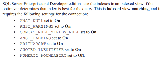
Effect: Forces the optimizer to use an index from the indexed view instead of expanding the view into its definition.
Example outcome (Listing 10-28): A query using NOEXPAND on a view yields a smaller, faster plan (e.g., reduced join count).
Example impact (Listing 10-28):
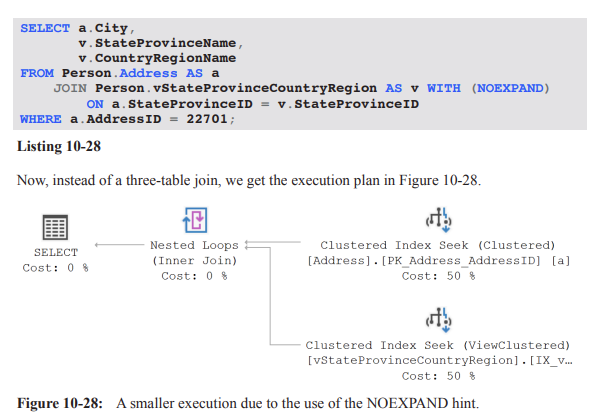
Query: SELECT a.City, v.StateProvinceName, v.CountryRegionName FROM Person.Address AS a JOIN Person.vStateProvinceCountryRegion AS v WITH (NOEXPAND) ON a.StateProvinceID = v.StateProvinceID WHERE a.AddressID = 22701;
Observed result: Plan with fewer joins; improved performance reported (e.g., from 189ms to 162ms and reads dropping from 6 to 4.
Important caveat: benefits are not guaranteed; always test, as improvements are workload-dependent.
SELECT a.City, v.StateProvinceName, v.CountryRegionName
FROM Person.Address AS a
JOIN Person.vStateProvinceCountryRegion AS v WITH (NOEXPAND)
  ON a.StateProvinceID = v.StateProvinceID
WHERE a.AddressID = 22701;
INDEX() hints
Purpose: Force the use of a specific index on a table during plan generation.
Syntax options:
WITH (INDEX(2)) — specify index by its numeric position (as numbered in sys.indexes). Note: 0 and 1 have special effects:
0 forces a scan of the clustered index or heap, depending on structure.
1 forces either a scan or a seek on a clustered index; it will error on a heap.
WITH (INDEX (IndexName)) — specify index by its name (recommended, since index numbers can change).
You can include multiple index specifications inside a single INDEX() hint to force the optimizer to consider multiple indexes in a particular order (e.g., INDEX (IndexName1, IndexName2)).
Important constraints:
Only a single INDEX() hint is allowed per table, but you can list multiple indexes inside that single hint to force an intersection and order.
This does not guarantee that only these indexes will be used, but it heavily biases the optimizer toward using them in the listed order.
Demos (Listing 10-29 to 10-31):
Simple example: forced multiple indexes on a single table to simulate an index-join scenario.
Demonstrates how the plan can change to reflect the specified index usage.
Practical example (Listing 10-34): forcing a specific index on HumanResources.Department using INDEX(PKDepartmentDepartmentID)
Query before hint uses an Index Seek on Department.
After hint: The plan shows a Clustered Index Scan (using the cluster key PKDepartmentDepartmentID) replacing the earlier Index Seek.
Performance impact observed in the example: execution time drops from 217 ext{ ms} to 103 ext{ ms}; reads remain roughly the same at 1042.
Key takeaway: Forcing a particular index can improve performance if the chosen index leads to a cheaper plan; however, the total reads may not always decrease, and plan shape can still change due to the forced index.
Practical guidance:
Use INDEX() hints to steer the optimizer when you have strong, evidence-based reasons (e.g., known expensive index seek patterns that the optimizer consistently misorders).
Always test with representative workloads and under load to ensure benefits are real.
Prefer naming the index in the hint to avoid reliance on index ordering, which can change over time.
-- Demonstration of INDEX() hint usage
SELECT isa.ID, isa.ColumnA, isa.ColumnB, isa.ColumnC
FROM dbo.IndexSample AS isa WITH (INDEX(FirstIndex, SecondIndex, ThirdIndex));
Demonstration: Practical example of forced index usage (Listing 10-34)
Context: Query selecting department Name, Employee JobTitle, and concatenated LastName, FirstName.
Original plan (Listing 10-33): Index Seek and Clustered Index Seek operators connected by Nested Loops.
With hint (Listing 10-34): Use INDEX(PKDepartmentDepartmentID) on HumanResources.Department to force the clustered index usage for that table.
Observed plan change (Figure 10-30): Clustered Index Scan on the targeted index replaces the prior index Seek. This aligns with forcing the optimizer to use the specified index, potentially changing the plan shape.
Performance outcome:
Execution time improved from 217 ext{ ms} to 103 ext{ ms}.
Overall reads remained approximately the same: 1042 reads.
The improvement demonstrates how index choice can affect plan efficiency, even when total reads don’t dramatically drop.
Practical takeaway:
Forcing an index via INDEX() can yield meaningful runtime improvements if the chosen index better matches the query pattern and data distribution.
Always validate across representative workloads and observe locking behavior, concurrency, and IO patterns, not just time.
Best practices and cautions on hints
Hints should be used sparingly and primarily for proven performance issues or architectural decisions.
Overuse or misuse can lead to suboptimal plans, regressions under load, or locking/contention issues.
Always test under realistic workloads and on representative data distributions.
Consider incremental changes: compare plans with and without hints, and monitor metrics such as:
Execution time (t),
Logical reads ( R ),
Physical reads, and
CPU time.
For table hints that affect locking strategies, be mindful of potential data integrity implications.
When using NOEXPAND with indexed views, ensure the connection settings align with the requirements listed (ANSINULL, ANSIWARNINGS, CONCATNULLYIELDSNULL, ANSIPADDING, ARITHABORT, QUOTEDIDENTIFIER, NUMERICROUNDABORT).
Documentation and reference:
Listing 10-27 demonstrates the syntax for applying hints via the WITH clause.
Listings 10-28 through 10-34 provide concrete examples of NOEXPAND, INDEX(), and specific index forcing in real queries.
Quick reference: key numbers and outcomes mentioned
Original plan: 485 logical reads; 74 ext{ ms}; top input to final Nested Loops yielded 455 rows.
HASH hint scenario: reads drop to 34; time roughly 74.1\,\text{ms}; plan uses Hash Match with subsequent changes to Merge joins.
NOEXPAND scenario: reads drop from 6 to 4; time from 189\,\text{ms} to 162\,\text{ms}.
INDEX() scenario (Listing 10-34): execution time 103\,\text{ms} vs 217\,\text{ms} without the hint; reads ≈ 1042 in both cases.
References to the specific listings and figures
Listing 10-25: Original plan with optimizer-chosen joins (Figure 10-26).
Listing 10-26: Query with HASH hint; Figure 10-27 shows the new plan (Hash Match + Merge changes).
Listing 10-27: Syntax overview for WITH (hint, hint, …) after FROM TableName.
Listing 10-28: NOEXPAND example; Figure 10-28 demonstrates the smaller execution plan.
Listing 10-29: INDEX() with numeric index specifier (INDEX(2)).
Listing 10-30: INDEX() with index name (INDEX(IndexName)).
Listing 10-31: INDEX() with multiple indexes (INDEX(IndexName1, IndexName2)).
Listing 10-32: Quick demo creating a sample table and multiple indexes.
Listing 10-33: Execution plan using indexes chosen by the optimizer (baseline plan).
Listing 10-34: Execution plan with forced index choice (PKDepartmentDepartmentID); Figure 10-30.
Notes:
The material above is synthesized from the transcripts of Chapter 10: Controlling Execution Plans with Hints. It summarizes the key concepts, examples, and their implications for query tuning using hints in SQL Server. The notes retain the numerical results in LaTeX format as requested.
FORCESEEK and FORCESCAN: Controlling the join-access strategy
Objective of hints: allow a user or DBA to influence the optimizer's choice for execution plans
FORCESEEK and FORCESCAN are table hints that force the requested operator type (seek vs scan) without forcing a specific index
This is described as the opposite of an index hint: an index hint forces the index, but allows the optimizer to choose between scan or seek
Important caveat: hints are not guaranteed to improve performance; they can hurt, especially as data changes over time
Example: No WHERE clause leads to scans (Listing 10-35)
SELECT p.Name AS ComponentName,
       p2.Name AS AssemblyName,
       bom.StartDate,
       bom.EndDate
FROM Production.BillOfMaterials AS bom
JOIN Production.Product AS p   ON p.ProductID = bom.ComponentID
JOIN Production.Product AS p2  ON p2.ProductID = bom.ProductAssemblyID;
Observation: without a WHERE filter, the optimizer uses scans to read data from the involved tables
Supporting evidence: execution plan shows scans (Figure 10-31)
Rationale: in the absence of selective predicates, scans are typically cheaper than repeated index seeks on large joins
The text notes that this behavior is completely normal given the query structure
Highlight from the plan: the highest estimated cost among index operations is the scan on the BillOfMaterials table
Forcing a Seek: Using FORCESEEK (Listing 10-36)
SELECT p.Name AS ComponentName,
       p2.Name AS AssemblyName,
       bom.StartDate,
       bom.EndDate
FROM Production.BillOfMaterials AS bom WITH (FORCESEEK)
JOIN Production.Product AS p   ON p.ProductID = bom.ComponentID
JOIN Production.Product AS p2  ON p2.ProductID = bom.ProductAssemblyID;
Outcome of forcing a seek: the optimizer is constrained to use a Seek on the BillOfMaterials table, which also propagates changes to other operators in the plan
Plan changes observed (Figure 10-32):
The previous Scan on BillOfMaterials is replaced with a Seek
The Hash Match operator is replaced with a Nested Loops join
Performance impact observed:
Execution time increases from about T{ ext{baseline}} \,\approx\, 145\text{ ms} to about T{ ext{forced}} \,\approx\, 290\text{ ms}
Reads increase from R{ ext{baseline}} = 34 to R{ ext{forced}} = 1160 reads
This implies higher resource usage and potential contention under load
Numerical summary (approximate):
Time ratio: \frac{T{ ext{forced}}}{T{ ext{baseline}}} \approx \frac{290}{145} \approx 2.0
Read ratio: \frac{R{ ext{forced}}}{R{ ext{baseline}}} \approx \frac{1160}{34} \approx 34.1
Lesson: forcing a seek can degrade performance depending on data distribution, join strategy, and how the optimizer would have chosen to access data
FORCESCAN: Reversing the operation
The FORCESCAN operator can be used to convert a Seek into a Scan
Use cases: when a Seek-based plan is found to be slower than a Scan for a given workload or data distribution
Caution: as with FORCESEEK, apply FORCESCAN only with careful testing; unintended plan changes can hurt performance
Practical Guidance and Warnings
The optimizer generally makes excellent decisions; it is designed to handle a wide variety of data patterns
Hints should be used judiciously; they represent a form of manual intervention in the optimizer
Data changes over time mean that a hint plan that is optimal today may become suboptimal in the future
If hints are used:
Test them thoroughly before deployment
Document their usage so they can be revisited or removed later
Re-test after database growth, schema changes, or upgrades
Patches and service packs can alter optimizer behavior; revalidate queries after upgrades
Hints are more often harmful than helpful; they should be a last resort, not the default approach
The examples intentionally show both beneficial and detrimental outcomes to reflect real-world behavior
Key Concepts and Takeaways
FORCESEEK / FORCESCAN:
Force the operator type (seek vs scan) without fixing the index
Contrast with index hints that fix a specific index while leaving scan/seek choice to the optimizer
Index vs Operator Cost:
The optimizer weighs cost of different access methods; a seek is not inherently cheaper than a scan
Forcing a seek can eliminate a cheaper plan path if the data distribution makes scanning more efficient
Execution Plan Dynamics:
Changing the operator type can cascade into changes in join methods (e.g., Hash Match vs Nested Loops)
Plan changes can drastically affect time and I/O (reads)
Empirical Testing:
Always measure performance impact before and after applying hints
Consider under load scenarios to assess contention implications
Data Evolution and Upgrades:
As data grows or distributions shift, hints may lose their effectiveness
Upgrades can alter optimizer behavior; retest queries using hints after applying patches or service packs
Real-World Relevance and Connections
Hints relate to the broader principle of cost-based optimization versus manual intervention
In production systems, hints should be treated as contingent adjustments, not permanent fixes
This example illustrates how a seemingly small change (forcing a seek) can have a large, unintended impact on throughput and resource usage
The discussion aligns with the broader theme of balancing performance tuning with maintainability and forward compatibility
Summary of Implications
Hints are powerful but risky: they can either improve or degrade performance
Always prefer letting the optimizer make decisions; resort to hints only when you have clear, measured evidence
Documentation and periodic re-evaluation are essential for long-term stability
Post-upgrade retesting is critical to account for potential changes in optimizer behavior
The goal is reliable performance with maintainable plans, not short-term gains from forcing a particular operator