AP Calculus BC Unit 9 Study Guide: Parametric Equations, Polar Coordinates, and Vector-Valued Functions

Parametric Equations: Representing Curves with a Parameter

A parametric equation describes a curve by giving both coordinates as functions of a third variable called a parameter (often time). Parametric functions are especially useful for showing the position of an object over time or describing curves that are awkward or impossible to write as a single function y=f(x).

Instead of thinking “%%LATEX1%% depends on %%LATEX2%%,” you think “both %%LATEX3%% and %%LATEX4%% depend on %%LATEX5%%,” where %%LATEX6%% plays the role of the independent variable:

x=f(t)

y=g(t)

Here, %%LATEX9%% and %%LATEX10%% are dependent and time/parameter t is independent.

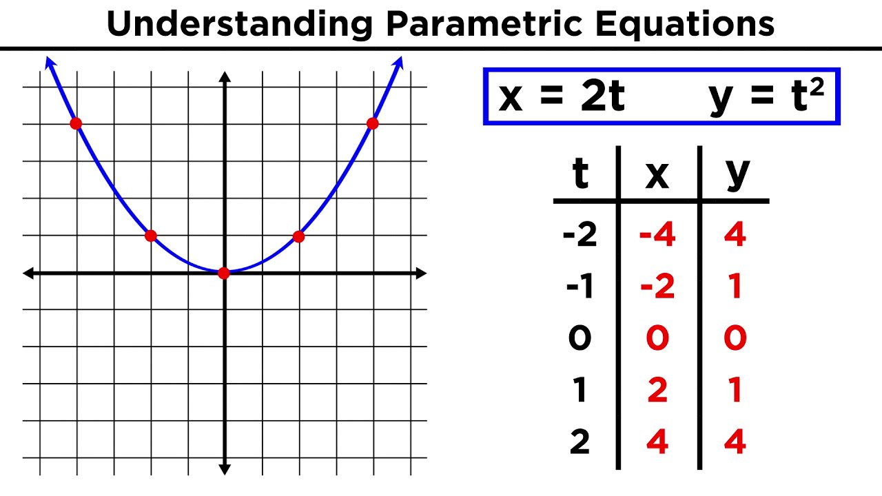
How parametric curves are traced (and why direction matters)

A single geometric curve can be traced in different ways depending on how t runs. The direction of tracing is part of the parametric description. Two different parametric pairs might generate the same set of points but in opposite directions or at different speeds.

To understand what the curve looks like, you can:

1. Pick values of %%LATEX13%%, compute points %%LATEX14%%, and plot them.
2. Eliminate %%LATEX15%% algebraically (when possible) to relate %%LATEX16%% and y directly.
3. Use technology to graph parametric equations directly.

Eliminating the parameter (when possible)

Sometimes you can solve for t from one equation and substitute into the other, converting the parametric curve into a Cartesian equation. This can help identify the curve (circle, parabola, etc.) and find restrictions.

Important caution: even if you eliminate t successfully, you may lose information about:

• which portion of the curve is traced
• the direction of motion
• how many times the curve is traced

Example 1: A circle from parametric equations

Suppose

x=3\cos(t)

y=3\sin(t)

Using \cos^2(t)+\sin^2(t)=1,

x^2+y^2=9\cos^2(t)+9\sin^2(t)

x^2+y^2=9

So the curve is the circle of radius %%LATEX25%% centered at the origin. If %%LATEX26%% increases from %%LATEX27%% to %%LATEX28%%, the circle is traced once counterclockwise.

Example 2: Same curve, different tracing

If you instead use

x=3\cos(2t)

y=3\sin(2t)

then as %%LATEX31%% goes from %%LATEX32%% to %%LATEX33%%, the angle %%LATEX34%% goes from %%LATEX35%% to %%LATEX36%%, so the circle is traced twice.

Exam Focus

• Typical question patterns
  • Identify the curve by eliminating t (and describe what portion/direction is traced).
  • Determine where the curve starts/ends for a given t-interval.
  • Recognize standard parametric forms (especially circles using sine and cosine).
• Common mistakes
  • Eliminating t and forgetting to state the correct domain or portion traced.
  • Ignoring direction: many AP questions expect “increasing t traces the curve from ___ to ___.”
  • Assuming a curve is traced once when it may be traced multiple times due to frequency changes like \cos(2t).

Calculus with Parametric Equations: Slopes, Tangents, and Concavity

Once you can represent a curve parametrically, you want calculus tools: slopes of tangents, rates of change, and concavity. The key idea is that %%LATEX42%% and %%LATEX43%% both depend on t, so derivatives come from the chain rule.

First derivative: finding dy/dx

If

x=x(t)

y=y(t)

differentiate each with respect to t:

\frac{dx}{dt}=x'(t)

\frac{dy}{dt}=y'(t)

As long as dx/dt\neq 0, the slope of the tangent line is

\frac{dy}{dx}=\frac{\frac{dy}{dt}}{\frac{dx}{dt}}

If %%LATEX53%% at a point, the ratio can “blow up.” That often signals a vertical tangent line (if %%LATEX54%%) or a cusp/corner-like behavior (if both derivatives are zero).

Tangent lines and normal lines

At a particular parameter value t=a:

1. Find the point \big(x(a),y(a)\big).
2. Compute the slope.

\left.\frac{dy}{dx}\right|_{t=a}=\frac{y'(a)}{x'(a)}

3. Write the tangent line (point-slope form):

y-y(a)=\left(\frac{y'(a)}{x'(a)}\right)(x-x(a))

A normal line is perpendicular to the tangent line. If the tangent slope is m (nonzero), the normal slope is

m_{\text{normal}}=-\frac{1}{m}

Second derivative: concavity for parametric curves

Concavity is about how the slope changes as x changes:

\frac{d^2y}{dx^2}=\frac{d}{dx}\left(\frac{dy}{dx}\right)

Rewrite %%LATEX63%% in terms of %%LATEX64%%:

\frac{d}{dx}=\frac{1}{dx/dt}\frac{d}{dt}

So

\frac{d^2y}{dx^2}=\frac{\frac{d}{dt}\left(\frac{dy}{dx}\right)}{\frac{dx}{dt}}

Example 1: Slope and vertical tangent

Let

x=t^2-4

y=t^3-3t

Compute derivatives:

\frac{dx}{dt}=2t

\frac{dy}{dt}=3t^2-3

So

\frac{dy}{dx}=\frac{3t^2-3}{2t}

A vertical tangent occurs when %%LATEX72%% and %%LATEX73%%. Here %%LATEX74%% gives %%LATEX75%%, and

\left.\frac{dy}{dt}\right|_{t=0}=-3

So there is a vertical tangent at t=0. The point is

x(0)=-4

y(0)=0

So the curve has a vertical tangent line at (-4,0).

Example 2: Second derivative via parameter

From

\frac{dy}{dx}=\frac{3t^2-3}{2t}

Differentiate with respect to %%LATEX82%% (for %%LATEX83%%). First rewrite:

\frac{dy}{dx}=\frac{3}{2}t-\frac{3}{2t}

Then

\frac{d}{dt}\left(\frac{dy}{dx}\right)=\frac{3}{2}+\frac{3}{2t^2}

Divide by dx/dt=2t:

\frac{d^2y}{dx^2}=\frac{\frac{3}{2}+\frac{3}{2t^2}}{2t}

Values of %%LATEX88%% where %%LATEX89%% are delicate; you usually analyze behavior around such points rather than plugging directly.

Exam Focus

• Typical question patterns
  • Find %%LATEX90%% at a particular %%LATEX91%% and write the tangent line.
  • Identify where the tangent is horizontal or vertical by setting %%LATEX92%% or %%LATEX93%%.
  • Compute d^2y/dx^2 at a parameter value and interpret concavity.
• Common mistakes
  • Setting %%LATEX95%% for horizontal tangents but forgetting the condition %%LATEX96%%.
  • Plugging into %%LATEX97%% at a point where %%LATEX98%% instead of recognizing a vertical tangent.
  • For %%LATEX99%%, differentiating %%LATEX100%% correctly but forgetting to divide by dx/dt.

Integrals with Parametric Curves: Area and Arc Length

Parametric equations also change how you compute areas and lengths. The unifying idea is that small changes in %%LATEX102%% produce small changes in %%LATEX103%% and y, and integrals add up those contributions.

Area under a parametric curve

For a standard function, area is

\int_a^b y\,dx

In parametric form, %%LATEX106%%. If %%LATEX107%% runs from %%LATEX108%% to %%LATEX109%% (or more generally from %%LATEX110%% to %%LATEX111%%), the signed area is

A=\int_{a}^{b} y(t)\frac{dx}{dt}\,dt

If %%LATEX113%% decreases over an interval (so %%LATEX114%%), this integral can be negative. On the AP exam, if the prompt says area, you typically report a positive value, which may require absolute values or splitting the interval.

Arc length of a parametric curve

Arc length is the distance along a curve. Because both %%LATEX115%% and %%LATEX116%% depend on t, you square both derivatives, add them, take the square root, and integrate over the parameter interval.

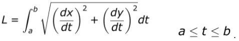
Over a small step dt:

dx\approx \frac{dx}{dt}dt

dy\approx \frac{dy}{dt}dt

So

ds\approx \sqrt{\left(\frac{dx}{dt}\right)^2+\left(\frac{dy}{dt}\right)^2}\,dt

and arc length from %%LATEX122%% to %%LATEX123%% is

L=\int_{a}^{b}\sqrt{\left(\frac{dx}{dt}\right)^2+\left(\frac{dy}{dt}\right)^2}\,dt

Example 1: Area under a parametric curve

Let

x=t^2

y=t^3

for 0\le t\le 1.

\frac{dx}{dt}=2t

So

A=\int_0^1 y(t)\frac{dx}{dt}dt

A=\int_0^1 t^3(2t)dt

A=\int_0^1 2t^4dt

A=\left.\frac{2}{5}t^5\right|_0^1

A=\frac{2}{5}

Example 2: Arc length that simplifies

Let

x=3\cos(t)

y=3\sin(t)

for 0\le t\le \pi (upper semicircle).

\frac{dx}{dt}=-3\sin(t)

\frac{dy}{dt}=3\cos(t)

Then

\left(\frac{dx}{dt}\right)^2+\left(\frac{dy}{dt}\right)^2=9\sin^2(t)+9\cos^2(t)

\left(\frac{dx}{dt}\right)^2+\left(\frac{dy}{dt}\right)^2=9

So

L=\int_0^{\pi}\sqrt{9}\,dt

L=\int_0^{\pi}3\,dt

L=3\pi

Exam Focus

• Typical question patterns
  • Set up (and sometimes evaluate) %%LATEX144%% as %%LATEX145%% on a given t-interval.
  • Set up arc length integrals (from %%LATEX147%% to %%LATEX148%%) and recognize when simplification is possible.
  • Interpret signed area vs. geometric area and decide whether to split intervals.
• Common mistakes
  • Using %%LATEX149%% instead of %%LATEX150%% for area under the curve (mixing up which variable is “height”).
  • Forgetting that decreasing x(t) can produce negative “area.”
  • For arc length, forgetting the square root or squaring only one derivative instead of both.

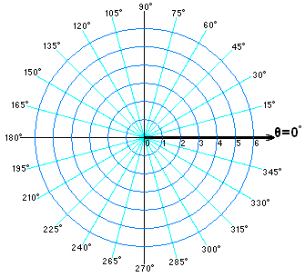
Polar Coordinates: Points and Curves in %%LATEX152%% and %%LATEX153%%

Polar coordinates replace Cartesian pairs %%LATEX154%% with %%LATEX155%%, where %%LATEX156%% is the (directed) distance from the origin (the pole) and %%LATEX157%% is the angle from the positive x-axis.

A polar equation typically has the form

r=f(\theta)

Polar form is often simpler for curves with circular or rotational symmetry (cardioids, roses, spirals).

Converting between polar and Cartesian

The basic relationships are

x=r\cos(\theta)

y=r\sin(\theta)

r^2=x^2+y^2

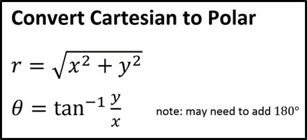
A subtle but important point is that a single point can have multiple polar representations:

\left(r,\theta\right)

and

\left(r,\theta+2\pi\right)

represent the same point, and

\left(-r,\theta\right)

represents the same point as

\left(r,\theta+\pi\right)

Negative r values are a common source of graphing confusion.

Recognizing common polar curves

Recognizing families helps you reason quickly:

• Circles can appear as %%LATEX168%% (circle radius %%LATEX169%% centered at the origin) or shifted forms like r=2a\cos(\theta).
• Rose curves often look like %%LATEX171%% or %%LATEX172%%.
• Cardioids / limacons often look like %%LATEX173%% or %%LATEX174%%.

Graphing strategy (conceptual)

When you graph %%LATEX175%%, you are asking: for each angle %%LATEX176%%, how far from the origin is the point?

1. Use key angles (like %%LATEX177%%, %%LATEX178%%, %%LATEX179%%, %%LATEX180%%) and symmetry angles.
2. Compute corresponding r values.
3. Plot and connect smoothly, paying attention to where r=0.

Symmetry tests (helpful but not magic):

• If f(-\theta)=f(\theta), symmetry about the polar axis.
• If %%LATEX184%%, symmetry about the vertical line %%LATEX185%%.
• If f(\theta+\pi)=-f(\theta), symmetry about the pole.

Example 1: Convert polar to Cartesian

Convert

r=4\cos(\theta)

Multiply both sides by %%LATEX188%% and use %%LATEX189%% and r\cos(\theta)=x:

r^2=4r\cos(\theta)

x^2+y^2=4x

Complete the square:

x^2-4x+y^2=0

\left(x-2\right)^2+y^2=4

This is a circle of radius %%LATEX195%% centered at %%LATEX196%%.

Example 2: Understanding negative r

Consider

r=2\sin(\theta)

When \theta=-\pi/2,

r=2\sin(-\pi/2)

r=-2

So the point at angle %%LATEX202%% with radius %%LATEX203%% is equivalent to radius %%LATEX204%% at angle %%LATEX205%%. This “flip” is why polar graphs can loop.

Exam Focus

• Typical question patterns
  • Convert between polar and Cartesian (often to identify a curve).
  • Sketch or interpret a polar curve, including where it hits the pole.
  • Use symmetry to justify integration bounds.
• Common mistakes
  • Treating r as always nonnegative and missing parts of the graph.
  • Converting incorrectly by substituting %%LATEX207%% instead of %%LATEX208%%.
  • Assuming one-to-one representation of points in polar form (forgetting equivalent representations).

Calculus in Polar Form: Slopes, Areas, and Arc Length

Polar calculus connects back to familiar ideas (slope, area, length), but you must account for the geometry of polar coordinates. A key reminder is that when differentiating polar relationships, you differentiate with respect to %%LATEX209%%, meaning you work with %%LATEX210%%.

Slope of a polar curve

Treat %%LATEX211%% as the parameter. If %%LATEX212%%, then

x=r\cos(\theta)

y=r\sin(\theta)

and

\frac{dy}{dx}=\frac{dy/d\theta}{dx/d\theta}

Using product rule,

\frac{dx}{d\theta}=\frac{dr}{d\theta}\cos(\theta)-r\sin(\theta)

\frac{dy}{d\theta}=\frac{dr}{d\theta}\sin(\theta)+r\cos(\theta)

So

\frac{dy}{dx}=\frac{\frac{dr}{d\theta}\sin(\theta)+r\cos(\theta)}{\frac{dr}{d\theta}\cos(\theta)-r\sin(\theta)}

Horizontal and vertical tangents follow the same numerator/denominator logic:

• Horizontal tangent: %%LATEX219%% and %%LATEX220%%
• Vertical tangent: %%LATEX221%% and %%LATEX222%%

Area enclosed by a polar curve

A thin sector of radius %%LATEX223%% and angle %%LATEX224%% has area

dA=\frac{1}{2}r^2d\theta

So area from %%LATEX226%% to %%LATEX227%% is

A=\frac{1}{2}\int_{\alpha}^{\beta}r^2\,d\theta

For the area between two polar curves (outer radius %%LATEX229%% and inner radius %%LATEX230%%), you subtract sector areas (this is the polar version of “top minus bottom,” but here it is outer minus inner):

A=\frac{1}{2}\int_{\alpha}^{\beta}\left(R^2-r^2\right)d\theta

Equivalently, if outer is %%LATEX232%% and inner is %%LATEX233%%:

A=\frac{1}{2}\int_{\alpha}^{\beta}\left(f(\theta)^2-g(\theta)^2\right)d\theta

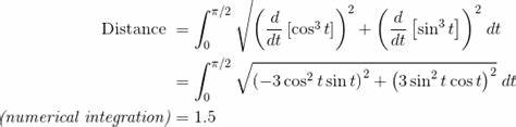
Arc length in polar form

From parametric arc length with parameter \theta,

L=\int_{\alpha}^{\beta}\sqrt{\left(\frac{dx}{d\theta}\right)^2+\left(\frac{dy}{d\theta}\right)^2}\,d\theta

This simplifies to the standard polar arc length form:

L=\int_{\alpha}^{\beta}\sqrt{r^2+\left(\frac{dr}{d\theta}\right)^2}\,d\theta

Example 1: Slope of a polar curve at a point

Let

r=2\cos(\theta)

Compute %%LATEX239%% at %%LATEX240%%.

\frac{dr}{d\theta}=-2\sin(\theta)

At \theta=\pi/3,

r=2\cos(\pi/3)

r=1

\frac{dr}{d\theta}=-2\sin(\pi/3)

\frac{dr}{d\theta}=-\sqrt{3}

Now

\frac{dx}{d\theta}=\frac{dr}{d\theta}\cos(\theta)-r\sin(\theta)

So

\frac{dx}{d\theta}=\left(-\sqrt{3}\right)\left(\frac{1}{2}\right)-\left(1\right)\left(\frac{\sqrt{3}}{2}\right)

\frac{dx}{d\theta}=-\sqrt{3}

And

\frac{dy}{d\theta}=\frac{dr}{d\theta}\sin(\theta)+r\cos(\theta)

\frac{dy}{d\theta}=\left(-\sqrt{3}\right)\left(\frac{\sqrt{3}}{2}\right)+\left(1\right)\left(\frac{1}{2}\right)

\frac{dy}{d\theta}=-1

Therefore,

\frac{dy}{dx}=\frac{-1}{-\sqrt{3}}

\frac{dy}{dx}=\frac{1}{\sqrt{3}}

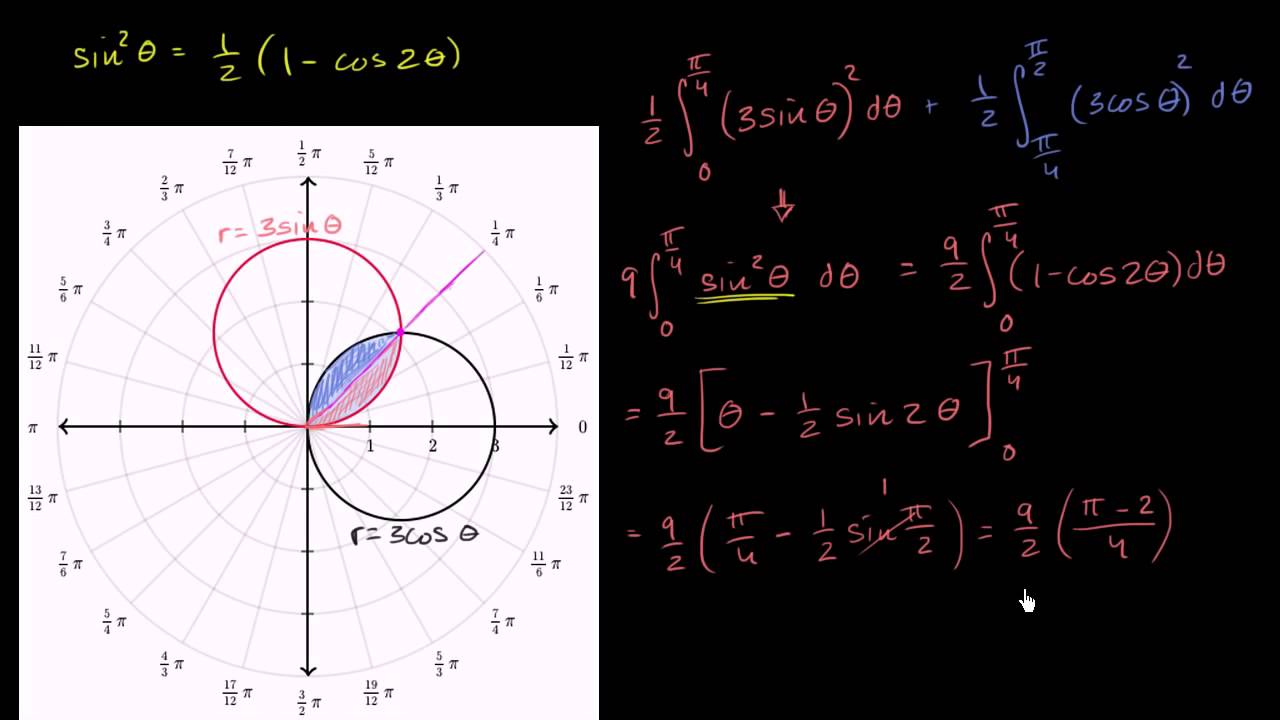
Example 2: Area inside a cardioid

Find the area inside

r=1+\cos(\theta)

over one full trace. This cardioid is traced once as %%LATEX256%% goes from %%LATEX257%% to 2\pi.

A=\frac{1}{2}\int_0^{2\pi}\left(1+\cos(\theta)\right)^2d\theta

Expand:

\left(1+\cos(\theta)\right)^2=1+2\cos(\theta)+\cos^2(\theta)

Use

\cos^2(\theta)=\frac{1+\cos(2\theta)}{2}

So the integrand becomes

\frac{3}{2}+2\cos(\theta)+\frac{1}{2}\cos(2\theta)

Integrate:

A=\frac{1}{2}\int_0^{2\pi}\left(\frac{3}{2}+2\cos(\theta)+\frac{1}{2}\cos(2\theta)\right)d\theta

Compute pieces:

\int_0^{2\pi}\frac{3}{2}d\theta=3\pi

\int_0^{2\pi}2\cos(\theta)d\theta=0

\int_0^{2\pi}\frac{1}{2}\cos(2\theta)d\theta=0

So

A=\frac{1}{2}\left(3\pi\right)

A=\frac{3\pi}{2}

Exam Focus

• Typical question patterns
  • Compute %%LATEX269%% for %%LATEX270%% at a given angle and write a tangent line.
  • Find area enclosed by a polar curve (or between two polar curves) by choosing correct intersection angles.
  • Set up arc length in polar form; sometimes evaluate if it simplifies.
• Common mistakes
  • Forgetting to square %%LATEX271%% in the area formula %%LATEX272%%.
  • Using incorrect bounds because the curve is traced twice or because r becomes negative.
  • Mixing up “outer minus inner” for area between two polar curves.

Vector-Valued Functions: Curves in the Plane via Vectors

Vector-valued functions map numbers (often time) to vectors. In the plane, a position vector is typically written as

\mathbf{r}(t)=\langle x(t),y(t)\rangle

This is the same information as parametric form, but the vector viewpoint makes motion ideas (position, velocity, acceleration) feel more natural.

Basic operations: differentiate and integrate component-wise

To derive velocity and acceleration (or to integrate back to position), you differentiate or integrate each component individually.

If

\mathbf{r}(t)=\langle x(t),y(t)\rangle

then

\mathbf{r}'(t)=\langle x'(t),y'(t)\rangle

and integration works the same way (component-wise), plus a constant vector.

The magnitude of \langle a,b\rangle is

\left|\langle a,b\rangle\right|=\sqrt{a^2+b^2}

Velocity, speed, and acceleration

For motion in the plane:

• Velocity is the derivative of position:

\mathbf{v}(t)=\mathbf{r}'(t)

• Speed is the magnitude of velocity:

\text{speed}=\left|\mathbf{v}(t)\right|

• Acceleration is the derivative of velocity:

\mathbf{a}(t)=\mathbf{v}'(t)=\mathbf{r}''(t)

A common trap is to confuse speed and velocity: velocity is a vector (direction matters), speed is a nonnegative scalar.

Integrating vector-valued functions (position from velocity)

If

\mathbf{r}'(t)=\mathbf{v}(t)

then

\mathbf{r}(t)=\int \mathbf{v}(t)dt

and you use an initial condition like \mathbf{r}(0) to find the constant vector.

Displacement vs. total distance traveled

AP Calculus BC loves the difference:

• Displacement from %%LATEX285%% to %%LATEX286%%:

\mathbf{r}(b)-\mathbf{r}(a)

Equivalently,

\int_a^b \mathbf{v}(t)dt

• Total distance traveled:

\int_a^b \left|\mathbf{v}(t)\right|dt

Example 1: Velocity, speed, and acceleration

Let

\mathbf{r}(t)=\langle t^2,3t-1\rangle

Then

\mathbf{v}(t)=\langle 2t,3\rangle

\left|\mathbf{v}(t)\right|=\sqrt{(2t)^2+3^2}

\left|\mathbf{v}(t)\right|=\sqrt{4t^2+9}

\mathbf{a}(t)=\langle 2,0\rangle

Example 2: Position from velocity and an initial condition

Suppose

\mathbf{v}(t)=\langle \cos(t),\sin(t)\rangle

and

\mathbf{r}(0)=\langle 2,-1\rangle

Integrate component-wise:

\mathbf{r}(t)=\left\langle \int \cos(t)dt,\int \sin(t)dt \right\rangle

\mathbf{r}(t)=\langle \sin(t)+C_1,-\cos(t)+C_2\rangle

At t=0:

\mathbf{r}(0)=\langle C_1,-1+C_2\rangle

Set equal to %%LATEX301%%, so %%LATEX302%% and C_2=0. Therefore,

\mathbf{r}(t)=\langle \sin(t)+2,-\cos(t)\rangle

Exam Focus

• Typical question patterns
  • Given %%LATEX305%%, find %%LATEX306%%, \mathbf{a}(t), and speed at a time.
  • Given %%LATEX308%% and %%LATEX309%%, find \mathbf{r}(t).
  • Compute displacement %%LATEX311%% versus total distance %%LATEX312%%.
• Common mistakes
  • Using \int \mathbf{v}(t)dt to compute total distance instead of integrating speed.
  • Forgetting the constant vector when integrating, then mishandling the initial condition.
  • Computing speed as \langle x'(t),y'(t)\rangle (a vector) instead of its magnitude.

Motion Along a Parametric or Vector Path: Connecting Concepts

Parametric equations, polar curves, and vector-valued functions are tightly connected:

• A parametric curve %%LATEX315%% is the same as %%LATEX316%%.
• A polar curve %%LATEX317%% becomes parametric by letting the parameter be %%LATEX318%% and using %%LATEX319%% and %%LATEX320%%.

Speed and arc length are the same idea

Parametric arc length was

L=\int_{\alpha}^{\beta}\sqrt{\left(\frac{dx}{dt}\right)^2+\left(\frac{dy}{dt}\right)^2}\,dt

But velocity is

\mathbf{v}(t)=\langle x'(t),y'(t)\rangle

so speed is

\left|\mathbf{v}(t)\right|=\sqrt{\left(x'(t)\right)^2+\left(y'(t)\right)^2}

Therefore,

L=\int_{\alpha}^{\beta}\left|\mathbf{v}(t)\right|dt

Arc length is literally total distance traveled.

When a particle changes direction

In two-dimensional motion:

• The particle is at rest when

\mathbf{v}(t)=\langle 0,0\rangle

• It speeds up or slows down based on how %%LATEX326%% changes; sometimes you are asked for %%LATEX327%%.

A useful identity for differentiating speed (when needed) comes from

\left|\mathbf{v}(t)\right|=\sqrt{\mathbf{v}(t)\cdot \mathbf{v}(t)}

Example 1: Distance traveled vs. displacement

Let

\mathbf{v}(t)=\langle 1,2t\rangle

from %%LATEX330%% to %%LATEX331%%.

Displacement:

\int_0^2 \mathbf{v}(t)dt=\left\langle \int_0^2 1dt,\int_0^2 2t dt \right\rangle

=\langle 2,4\rangle

Total distance:

\int_0^2 \left|\mathbf{v}(t)\right|dt=\int_0^2 \sqrt{1^2+(2t)^2}dt

=\int_0^2 \sqrt{1+4t^2}dt

This typically does not simplify with basic BC tools, so it may be left as an integral or approximated numerically, depending on the problem.

Example 2: Polar to parametric to compute a tangent slope

Given

r=2+\sin(\theta)

at a specific \theta, you can compute slope by converting to parametric:

x=(2+\sin(\theta))\cos(\theta)

y=(2+\sin(\theta))\sin(\theta)

Then differentiate both with respect to \theta and use

\frac{dy}{dx}=\frac{dy/d\theta}{dx/d\theta}

Exam Focus

• Typical question patterns
  • Translate a polar curve to parametric form to apply parametric derivatives.
  • Interpret arc length as distance traveled and connect it to speed.
  • Decide whether a question wants displacement (vector) or distance (scalar).
• Common mistakes
  • Using the arc length formula but integrating from the wrong parameter bounds (mixing %%LATEX342%% and %%LATEX343%% intervals).
  • Confusing displacement with distance traveled.
  • Differentiating polar-to-parametric conversions incorrectly (missing product rule on %%LATEX344%% or %%LATEX345%%).

Advanced Tangent Behavior: Horizontal and Vertical Tangents in Parametric and Polar Settings

AP Calculus BC often tests tangent behavior beyond “compute a derivative.” The core idea is always that slopes depend on a ratio, so the numerator and denominator matter separately.

Parametric horizontal and vertical tangents

For parametric curves:

\frac{dy}{dx}=\frac{dy/dt}{dx/dt}

• Horizontal tangent at t=a typically means

\frac{dy}{dt}(a)=0

and

\frac{dx}{dt}(a)\neq 0

• Vertical tangent at t=a typically means

\frac{dx}{dt}(a)=0

and

\frac{dy}{dt}(a)\neq 0

If both are zero, you need deeper analysis (cusp/corner, or a momentary stop).

Polar horizontal and vertical tangents

For polar curves, use

\frac{dy}{dx}=\frac{dy/d\theta}{dx/d\theta}

• Horizontal tangent when %%LATEX354%% and %%LATEX355%%
• Vertical tangent when %%LATEX356%% and %%LATEX357%%

Example: Finding horizontal tangents parametrically

Let

x=t^2+1

y=t^3-3t

Compute

\frac{dx}{dt}=2t

\frac{dy}{dt}=3t^2-3

Horizontal tangents require 3t^2-3=0:

t^2=1

t=-1,1

Check %%LATEX365%%: at %%LATEX366%%, 2t\neq 0, so both are valid.

Points:

At t=1:

x=2

y=-2

At t=-1:

x=2

y=2

So horizontal tangents occur at %%LATEX374%% and %%LATEX375%%.

Exam Focus

• Typical question patterns
  • Solve for parameter values where tangents are horizontal/vertical and give the corresponding points.
  • Determine whether a parameter value gives a true tangent line or a cusp (when both derivatives vanish).
  • For polar curves, find tangent behavior by working with %%LATEX376%% and %%LATEX377%%.
• Common mistakes
  • Finding t values correctly but forgetting to convert them into points on the curve.
  • Declaring “horizontal tangent” when %%LATEX379%% but %%LATEX380%% too.
  • In polar problems, trying to set dr/d\theta=0 for horizontal tangency (that is not the correct condition).

Putting It All Together: Multi-Representation Thinking (Parametric, Polar, Vector)

This unit is less about isolated formulas and more about flexibility: you’re expected to move between representations and choose efficient methods.

A notation connection table

A realistic modeling perspective

If you’re modeling motion:

• Vector form is often the cleanest because position, velocity, and acceleration are naturally vectors.
• Parametric form is essentially the same but can be convenient for slope/area setup.
• Polar form is ideal when motion is naturally described by an angle and a distance from a central point (satellites, radar sweeps, spirals).

Example: Recognizing equivalent descriptions

If you are given

\mathbf{r}(t)=\langle 4\cos(t),4\sin(t)\rangle

you can immediately interpret:

• It is parametric with %%LATEX393%% and %%LATEX394%%.
• Eliminating t gives

x^2+y^2=16

so it’s a circle of radius 4.

• Speed is constant because

\mathbf{v}(t)=\langle -4\sin(t),4\cos(t)\rangle

and

\left|\mathbf{v}(t)\right|=\sqrt{16\sin^2(t)+16\cos^2(t)}

\left|\mathbf{v}(t)\right|=4

Exam Focus

• Typical question patterns
  • Convert between representations (polar to parametric; parametric to Cartesian; vector to parametric).
  • Use the representation to compute a derivative/integral quantity (slope, area, distance).
  • Interpret motion context: position, velocity, acceleration, speed, displacement, distance.
• Common mistakes
  • Treating conversion formulas as interchangeable without checking what parameter is being used.
  • Missing that some curves are traced multiple times, which affects area bounds and graph interpretation.
  • Losing geometric meaning by focusing only on algebra (for example, not checking whether an “area” integral is signed).