Math

Day 1

Course information

If I have questions about the achieve app there is an explanatory session on Wednesday, 8/21 in BRWN 1152: 10 AM to 2 PM, I do not have to attend the whole session, its just a Q&A.

Supplemental Instruction Courses if necessary;

• Monday 6:30-7:20 PM SCHM 108

• Tuesday 6:30-7:20 PM SCHM 108

• Thursday 6:30-7:20 PM SCHM 108

These courses are led by Melissa Mancera, her office hours are Thursday 1:30-2:39 PM at Wiley C215 & Online via Zoom

Pre-Knowledge

Functions, these are equations that have an input (x) and an output (f(x)). The Domain is that total list of possible inputs and the Range is the total list of possible outputs.

Rules for the Natural Base (e^x)

• e⁰ = 1

• e^a+b = e^a * e^b

• e^a-b = e^a/e^b or e^a * e^-b

• (e^a)^b = e^{a * b}

Rules for the Natural Logarithm (ln)

• ln(1) = 0

• ln(e¹) = 1

• ln(ab) = ln(a) + ln(b)

• ln(a/b) = ln(a) - ln(b)

• ln(a^b) = bln(a)

Rules for Basic Trigonometry

SohCahToa

Sineθ = o/h

Cosineθ = a/h

Tangentθ = o/a

Cotangentθ = 1/Tanθ

Cosecantθ = 1/Sinθ

Secantθ = 1/Cosθ

Sin²θ + Cos²θ = 1

Tanθ = Sinθ/Cosθ

Unit Circle

This is a circle with a Radius of 1 that is Centered at the point (0,0). This includes finding a point on the circle using the angle, or finding the angle based off the point on the circle. Notable points include:

• At 60 degrees the point on the circle is (1/2,√3/2)

• At 45 degrees the point on the circle is (π/4,π/4)

• At 30 degrees the point on the circle is (√3/2,1/2)

Day 2

Limits

The mathematical concept of finding limits is the process of finding the value (y) that gets approached when moving the x-value closer to the desired input. There are instances where the exact output value is not the same as the value that is approached when getting closer to the desired input. Also, a limit may only exist when the limit exists from both the negative direction and the positive direction. If the limit found from either direction does not match, then the limit will be determined to not exist. There are 2 ways to find limits, the first is graphically, the second is numerically.

Graphically

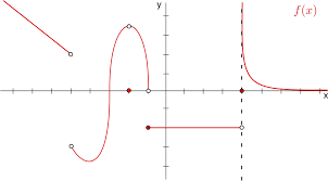
This is an example of what a graph could look like, it passes the vertical line test so it therefore is a function.

An example for this could be the limit at x = -5, from the negative side the value approaches y = 2, but from the positive side the value approaches y = -2. So, the limit does not exist in this instance.

However if we look at x = -2, from the negative side the value approaches y = 3.5, from the positive side the value approaches y = 3.5. So, Left side = Right side, therefore the limit does exist, even though the exact value for x = -2 is in fact y = 0.

Numerically

The other way to find limits is numerically, this is the process of plugging values that get closer to the desired input, until you can intuitively see the number that is being approached whether that be a number like 7 or infinity. The left side must still equal the right side in this instance however.

Analytically

Instead of the trial and error strategy of the numerical method, the analytical way saves much more time. The way to accomplish this is by using intuition to find the limit. First is to determine what is actually a function. A few examples of functions include:

• Polynomials

• Rational Functions

• Logarithms

• Exponentiation

• Trigonometry

They way to do this is to plug the limit directly into the function. If the solution is undefined there are a couple cases to look at.

Case 1

f(c) = nonzero/0

in this case the limit will be either positive or negative infinity

With examples like

lim(x→c) 1/(x-c)ⁿ = the limit is infinity if the exponent is even, it is DNE if the exponent is odd

Case 2

This is for the case with higher order polynomials, try to factorize the top and bottom as much as possible to get a easier problem to look at.

Piecewise function: This is a type of function that is made up of multiple different equations in different segments of the domain.

Another concept to consider with functions and limits is whether they have continuity or discontinuity.

A function is continuous if you have the ability to draw the full function without picking up the pencil. This even works for piecewise functions.

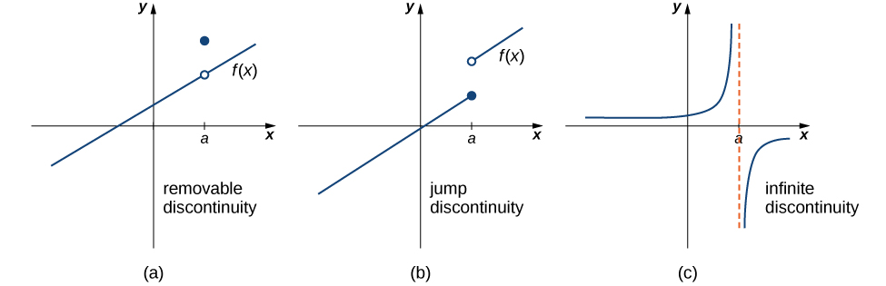
A function is discontinuous if there are breaks in the function (points where the line is not connected). There are 3 types of discontinuities:

• Jump Discontinuity

• Hole (removable) Discontinuity

• Vertical Asymptotes (Infinite) Discontinuity

Derivative

A derivative represents the rate at which a function is changing at any given point. In calculus, it is defined as the limit of the average rate of change of the function as the interval approaches zero. Mathematically, for a function ( f(x) ), the derivative is denoted as ( f'(x) ) or (df/dx).

One way to find the average rate of change or (slope) at any given point could be to find the tangent line. This could be found by using previous knowledge on limits. By finding the slope between 2 points as the point approaches the desired point.

A derivative is usually shown by either f’(x) or dy/dx

Another, much easier way to find a tangent line is by using the formula;

To find the tangent line to a curve at a specific point, follow these steps:

1. Identify the Function: Start with the function ( f(x) ).

2. Find the Derivative: Calculate the derivative ( f'(x) ) to determine the slope of the tangent line.

3. Evaluate the Derivative: Substitute the x-coordinate of the point of tangency into ( f'(x) ) to find the slope ( m ).

4. Find the Point: Determine the y-coordinate by evaluating ( f(x) ) at the same x-coordinate.

5. Use Point-Slope Form: Apply the point-slope formula ( y - y_1 = m(x - x_1) ) to write the equation of the tangent line, where ( (x_1, y_1) ) is the point of tangency.

This results in the equation of the tangent line.

Basic Rules of Differentiation

Power Rule

If ( f(x) = xⁿ ), then ( f'(x) = nx^n-1)

This formula works for all real numbers, a couple of basic rules of differentiation to understand are

• (1/f(x))’ ≠ (1/f’(x))

• f(θ) sin(θ) → f’(θ) cos(θ)

• f(θ)cos(θ) → f’(θ) -sin(θ)

• f(x) e^x → f’(x) e^x

Product Rule

(f(x)g(x))’ → f’(x)g(x) + f(x)g’(x)

Quotient Rule

(f(x)/g(x))’ → (g(x)f’(x) - f(x)g’(x))/(g(x))²

Chain Rule

(g∘f)(x) = g(f(x))

(g(f(x))’ = g’(f(x))(f’(x))

Mostly deals with examples for a binomial with an exponent

f(θ) sec(θ) → f’(θ) sec(θ)tan(θ)

f(θ)cot(θ) → f’(x)-csc²(θ)

f(θ) csc(θ) → f’(x)-csc(θ)cot(θ)

f(θ) tan(θ) → f’(x) sec²(θ)

(ln(x))’ = 1/x

Differentiation problems can either be in the implicit form or explicit form

Implicit: y = f(x)

Explicit: 1 = y² + x²

For Explicit differentiation treat y as a function of x and use the chain rule to isolate the derivative of y

Related Rates

Related rates are a method in calculus used to find the rate at which one quantity changes in relation to another. This technique often involves using implicit differentiation to relate the rates of change of different variables in a problem.

Example of a Related Rates Problem

Problem:

A balloon is being inflated and is rising into the air. The radius of the balloon is increasing at a rate of 2 cm/min. How fast is the height of the balloon rising when the radius is 10 cm?

Solution Steps:

1. Identify Variables:

   • Let ( r ) = radius of the balloon (cm)

   • Let ( V ) = volume of the balloon (cm³)

   • Let ( h ) = height of the balloon (cm)

2. Volume Formula: [ V = \frac{4}{3} \pi r^3 ]

3. Differentiate with respect to time ( t ): [ \frac{dV}{dt} = 4\pi r^2 \frac{dr}{dt} ]

4. Substitute known values:

   • ( \frac{dr}{dt} = 2 ) cm/min

   • ( r = 10 ) cm

5. Calculate ( \frac{dV}{dt} ): [ \frac{dV}{dt} = 4\pi (10^2)(2) = 800\pi \text{ cm}^3/\text{min} ]

6. Find height rate if needed (additional context required).

This problem illustrates how to relate the rates of change of different quantities.