Pearson's Chi-Square

Pearson Chi-Square (for Goodness of Fit)

Codes: Topic Color: #fffb89 ; Observed Categorical frequencies (O): #9bc8ff ; Expected Frequencies (E): #ffbdbf ; Examples: green ; Simplified: #ebc3ff

About Pearson’s Chi-Square

Pearson’s Chi-Square is a type of categorical data analysis

Assumptions of the Pearson Chi-Square Goodness of Fit Test:

• Categorical Data: The data must be in the form of frequencies (counts) for different categories or groups.

• Independence of Observations: Each observation must be independent of all other observations. One subject's inclusion in a category should not influence another's.

• Expected Frequencies:

  • The expected frequency ($E$) for each category should be sufficiently large.

  • A common rule of thumb is that no more than 20% of categories should have an expected count less than 5 and no category should have an expected count less than 1

  • If this assumption is violated, the chi-square approximation to the sampling distribution may be inaccurate.

• Random Sample: The sample should be a simple random sample from the population of interest.

Categorical Data Analysis

    What is categorical analysis?

• Categorical analysis: this is the examination of a possible relationship between categorical variables

    What are categorical variables?

• Categorical variables: these are variables that represent specific groups

  • Simplified: So, a categorical variable is one where a person’s answer places them into separate group and categories

                   (e.g., eye color *green*, *blue*, *brown*; gender *male* vs *female*)

        Categorical Variable Rules

        1) They must be mutually exclusive

             i. The subject have to be in only one category

        2) They must be ordered

             ii. Categories can be ordered from least to greatest

Purpose of Pearsons Chi-Square 

So, what is this tests purpose?

    1. You only have one variable and it is categorical

    2. The categories are observed not assigned

    3. Interested in how participants are distributed across different categories

        (e.g., is one category more prevalent than the other categories)

Example Purpose (research) Question:

Are there locations for education abroad programs that are more attractive than others?

The Overall Purpose:

The purpose is really to see if observed categorical frequencies (O) (what people choose to answer about location attraction) significantly differ from expected frequencies (E) (whatever data that says to expect a certain answer or data that wants us to assume it’s equal if we don’t have data to compare to) based on a null hypothesis.

• Simplified: Basically Chi-Square sees how well an observed data (on distribution) matches the expected data (data we expect from the scenario on the distribution).

When to use Pearson’s Chi-Square

    When will we use the Pearsons Chi-Square?

• We use this if we want to see if a sample distribution matches:

        A known population distribution OR a theoretically uniform distribution.

    How do we determine which distribution to compare your sample to?

    1) Use Known Distribution ➡ when research or records already give you         percentages to expect

    2) Use Uniform Distribution ➡ when you don’t have prior knowledge or a given expectation and theory says outcome should come out equal

    **Don’t worry, we compare at the end after we get our chi-square #

Before we jump into an example problem, let’s discuss observed frequencies, expected frequencies, and null hypothesis

Frequencies (Observed & Expected) & Null Hypothesis

Observed and Expected Frequencies

    What are Observed Frequencies (O)?

• This is the number of counts that we observe or get for each category based on our research data

  • Simplified: You can just think of it as the data we collected from each group

  • E.g., Say we surveyed 300 college students and the observed frequencies are as follows:

    • 200 students prefer Greece (200 is the Observed Freq)

    • 50 students prefer Japan (50 is the observed freq)

    • 50 students prefer Portugual (50 is the observed freq)

    Null Hypothesis

• Basically you want to figure out what the probability would be for group membership if the null is true

  • The null must therefore be some expected portion for each category

    • Remember we asked earlier when will we know whether to compare to a uniform distribution or known distribution? Well this is where it is relevant.

      • Some expected portion is either a number we get from a theoretical distribution (the uniform one) or an already known number to compare it to.

  • E.g., Say we want to know whether the three locations are equally preferred (uniform)

    • This means 33% of participants should be in each category for them to be equally distributed among categories

    • It’s 33% because 33% of 300 students = 300/3 (categories) = 100 students per category 

What are Expected Frequencies (E)?

•   These are the frequencies we should observe if the hypothesis is true 

  • Simplified: the null would be true if each category had 100 students

  • E.g., In our example we expect there will be 33% of the sample in each category therefore we could expect our categories to look like this 

    • Greece = 100 students 

    • Japan = 100 students

    • Portugal = 100 students 

How Pearson Chi-Square Works 

    Important to know the hypotheses 

• If the Null is True → then the observed frequency (O) should be the exact same as the expected frequency (E) 

• If the Null is False → then there should be a difference between observed frequency (O) and expected frequency (E) 

    ★Therefore, to figure this out we need to quantify the difference (find the amount of difference) between         (O) and (E) and compute the p-value for it 

The Test Steps for Chi-Square

Chi-Square Formula

• $\chi^2$ = the Pearson Chi-Square test statistic.

• $\sum_{i=1}^{k}$ = the sum across all $k$ categories.

• $O_i$ = the observed frequency (count) for the $i$-th category.

• $E_i$ = the expected frequency (count) for the $i$-th category under the null hypothesis.

Step 1. Take the Difference Between O & E

Since the null says we should expect that each category is equally preferred we would subtract 100 from each

• We take 100 out because that is how much we expected each category to have under the null hypothesis

        Example: Greece, Japan, Portugal

        Blue = observed scores; purple = expected scores

        —Greece: 200 - 100 = 100

        —Japan: 50 - 100 = -50

        —Portugal 50 - 100 = -50

Step 2. Now Square Each of These

        —Greece: $100^2$ = 10,000

        —Japan: $-50^2$ = 2,500

        —Portugal: $-50^2$ = 2,500

Step 3. Adjust for Sample Size

• Before we sum the squared values or continue forward we want to adjust for sample size

                                    But Why?

• Because the same raw difference means different things based on what the sample size is

  • E.g.,

    • O - E = 5 in a sample of 10

  •                        vs

    • O - E = 5 in a sample of 1000

    Actual Start of Step 3:

• Therefore to account for sample size, we divide the squared difference by the expected frequency

        —Greece: $\frac{100^2}{100}$ = 100

        —Japan: $-\frac{50^2}{100}$ = 25

        —Portugal: $-\frac{50^2}{100}$ = 25

Step 4. Calculate the Statistic Place on The Sampling Distribution

• You get this statistic by adding up all the values just calculated!

        —Greece:100

        —Japan: 25

        —Portugal: 25

         = 100 + 25 + 25 = 150

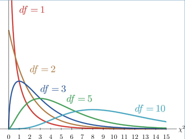
Step 5. Review the Chi Square Distribution

• The Chi-Square Distribution is not just 1 curve—its a family of curves!

• These curves have all different shapes because they are determined by the degrees of freedom—or really the amount of categories you have

• Also notice the lowest it can go is 0 and that is because it can’t be negative

Step 6. Degrees of Freedom

• Degrees of freedom are always the number of independent pieces of information you got going on —basically the number of categories - 1.

  • In our example we have 3 categories: Greece, Japan, Portugal

  • Therefore: 3 - 1 = 2

Step 7. Significance Level ($\alpha$ = .05) and Critical T

• Significance level or alpha is usually always .05 or 5%

  • This means you want to know the cutoff for the top 5% of the chi-square curve.

  • This indicates only really rare results (lying at 5% or less) will make us reject the null.

• Critical t (look up on chi square table)

  • Crit t is like a fence saying anything past here indicates it’s unusual meaning we reject null cause something is happening

  • For ours look for df of 2 and then the alpha .05

    • You will then find the fence or crit-t is standing at 5.991 (marked with red dotted line)

    • BUT our Chi square statistic was 150…that’s WAY more than 5.991 and would sit way futher than the 20 on that graph!

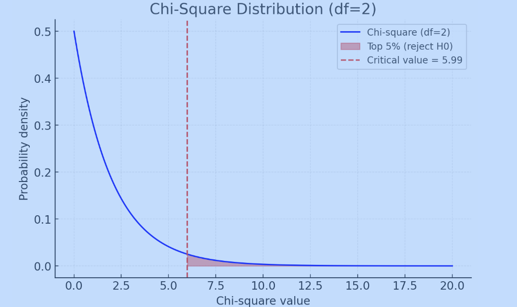
If our statistic falls before the red line that says there is no difference (null is true), but if our chi-square statistic is more than our critical t value, that indicates a difference (people prefer one of the locations more than the others)!