Start of statistics

Null hypothesis:

no need for a null hypothesis under the research design

• No difference between groups/conditions

• Numerical differences caused by random noise

• Not caused by the independent variable

• The default position that your experiment is seeking to falsify

  • benefit in proving null hypothesis sometimes

Alternative Hypothesis:

• A difference/relations exists between groups/conditions

• Numerical differences are real/non-random

• differences seen are because of the things you are changing

Experimental power:

• Your ability to detect an effect of a certain size

• Underpowered studies will leave you unable to detect small effects

  • sometimes you don’t have enough elite athletes to analyze the effect of one small supplement, cant power the study enough to show statistically meaningful effects

• Most effects you are likely to examine are probably pretty small, given that you are examining slight adaptations of established paradigms.

• Easiest way to ensure you have enough power is to test plenty of people

  • No such thing as ‘too much power’

Type 1 error:

• incorrect rejection of a true null hypothesis

• Usually, a type 1 error leads one to conclude that a supposed effect or relationship exists when in fact it does not!

• The level of type 1 error we are willing to risk is called our α (alpha) level

• Typically, we set our alpha to 0.05, meaning type 1 errors will occur 5% of the time (1 in 20)

t test comparing 2 means

Type II error

• The failure to reject a false null hypothesis

• Usually, a type 2 error leads one to conclude that an effect or relationship does not exist, when in fact one does

• The level of type 2 error we are willing to risk is called our β (beta)

• f we power our study to 0.8, this means our beta is 0.2 and we have a 20% chance of a type 2 error

when the risk of these error increase we can control for them

In context

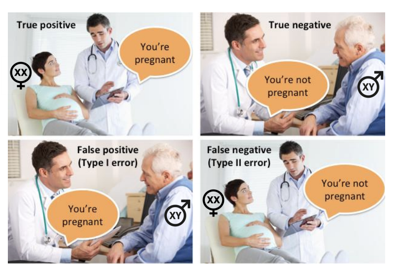
A doctor is diagnosing whether an individual has an illness

• Type 1 error is when a diagnostic test suggests someone is sick when they in fact are NOT sick at all (false positive)

• Type 2 error is when a diagnostic test suggests someone is healthy when they are actually sick (false negative)

Statistical tests are based on the assumption that all variance is due to two things:

• True effects

• Random factors

All about the decision of the person interpreting the test

• Type I error: decide there is a true effect, when random factors actually produced observed effect.

• Type 2 error: decide there is no effect, when random factors have masked true effect.

Null Hypothesis:

• In isolation, p values cannot demonstrate that there are no difference between conditions

• p>0.05 does not allow you to accept the null hypothesis

• p>0.05 does not tell you that a manipulation has no effect

• p>0.05 does not tell you that the scores in two conditions are the same as one another

it can not do any of that, it does give an indication of the likely hood that what is happening has happened by chance.

• a probability value

• what is the probability that this has happened by chance?

  • P value of 0.04 means you can say what is happening is due to the manipulation but there is a 96% probability that what is happening is because of the manipulation and not because of random other effects that come from the data.

a p value of 0.06 is not statistically different, there is no statistical effect of the independent variable, there could be something happening = partial pita square

Range of reasons why p>.05:

• No actual effect

• Type 2 errors oLack of power (i.e., too small a sample to detect an effect of a certain size)

• Inadequate variability within independent variable

• Measurement error

• Nuisance variables (things that you might not know of, example; drinking the day before a test

• A null finding should not be considered a ‘failure’, especially in your dissertation.

  • it is hard to discuss why you have no statistical evidence, taking other literature and comparing things would benefit.

• No extra marks awarded for significant differences!

Often difficult to publish null-findings

• Publication bias – the tendency for significant results to be published at the expense of nonsignificant results: systematic reviews have an element of publication bias in them

• an anova with a p vl of less than 0.05, you need to talk about an effect, they show the effects

• post op t test show differences between two means

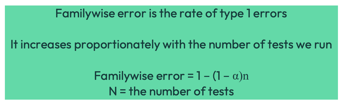
FAMILYWISE ERROR

why has a study not shown an effect when all of the previous studies have?

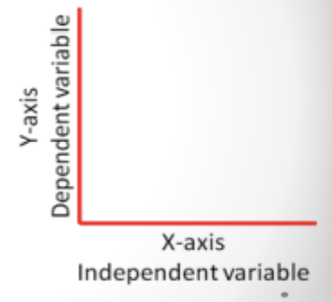
• We use experimental designs to try to establish cause and effect

• We manipulate independent variables and measure dependent variables

a repeated measures anova and an independent anova would be better

more t test increases the chances of showing a statistical effect when there are no effects there

If we are comparing two groups of scores

• E.g. Drug A vs. control

• Use a t test

If we have more than two groups of scores

• E.g. Drug A vs. Drug B vs. Control

• Run a few t-tests? NO

• E.g. Compare drug A to Drug B, Drug A to control and Drug B to control

each test we run inflates the familywise error rate

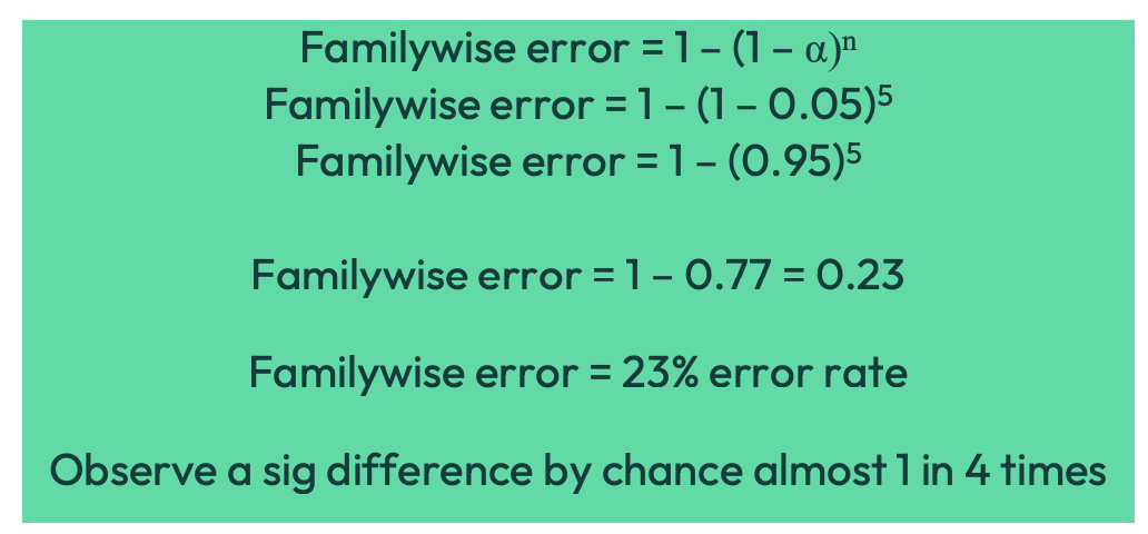
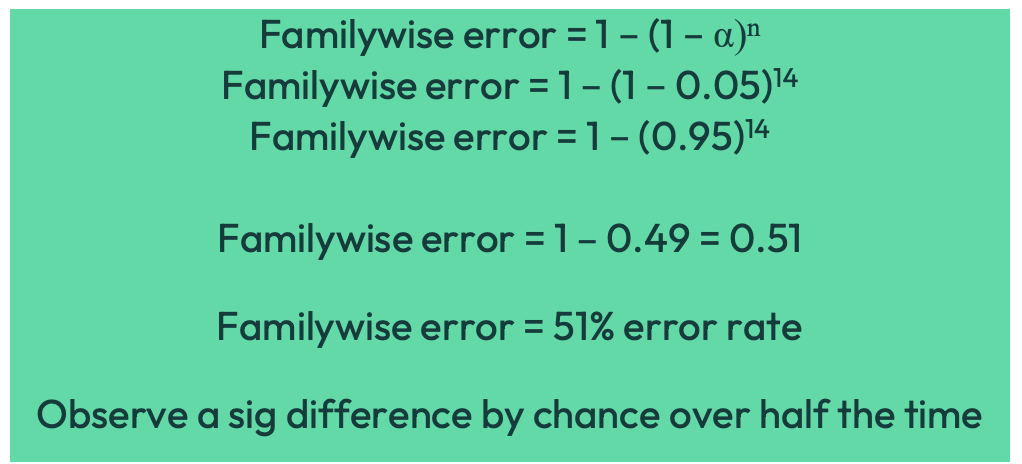
corrections: is it possible to mathematically account for a familywise error

corrections such as:

• Bonferroni

• Turky’s HSD

• Holm

• Scheffe

All of these corrections reduce your ability to detect a true effect

• i.e. they lower your experimental power and increase your chance of making a type 2 error

• The solution?

  • One-way independent ANOVA

Analysis of variance - ANOVA between each of the columns of data

• M = typically used to signify the mean of a group of scores

• df = degrees of freedom

• g = the number of groups

• N = total number of scores

• n = number of scores in each group

• SS = sum of squares

• MS = means square (variance)

• ∑= the sum of

One-way independent ANOVA:

• Compares three or more groups using a single statistical test

• Controls the familywise error rate

• Maintains statistical power compared with multiple t-tests

• Tells you whether the factor has a significant overall effect

  • one factor, for example steroids, therefore we do a one-way

  • no steroid, low dose, high dose (condition), time is also changing, therefore one would do a 2 way anova. The independant variable is the factor

• Post hoc tests are then used to identify which groups differ

  • effect is with factor, differ is with post op test, suggesting t test after the anova

Assumptions:

• The samples are unrelated to each other (independent)

  • Like an independent t test

• The data is interval/ratio scale

  • For ordinal data use non-parametric Kruskal-Wallis test

• Data is normally distributed

  • ANOVA quite robust to violations of normality

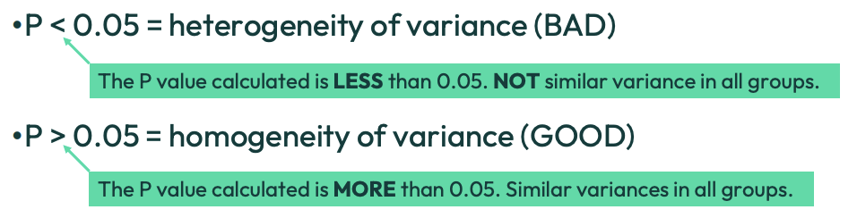
Further assumptions:

• Homogeneity of variance

• Similar variances in all groups

• Measured using Levene’s test

Similar variances in all groups, for ANOVA the levenes test is done, for repeated measures this tests for sarisity, one way you can identify if its a independent or a repeat measures anova. Outputs are something important to include in the exam

ANalysis Of VAriance

• In ANOVA tables, variance is called ‘Mean Square’ (MS)

• Effect/treatment variance

• Error variance

• Mean square error (MSE)

• Variance is visually demonstrated in graphs by error bars

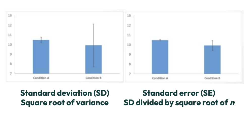
Standard error will always be smaller than standard deviation

ANOVA:

• ANOVA asks how successful the experimental manipulation has been in comparison to the natural variability that exists

  • natural variability between individuals and in the person on the other end, person collecting the information.

• Compares the type of variance you want (effect variance) with the type of variance you do not want (error variance)

  • we want to minimize error variance as much as possible, this is why you control as much as you can in a lab environment

• This ratio between wanted (effect) and unwanted variance (error) is called the F-ratio

Error variance (MSE)

• Measurement error

• Always present because variables cannot be measured perfectly

• Individual differences: always present in anything that you are measuring

• Always present because scores might naturally vary from person to person

• For independent ANOVA, the error variance (MSE) always occurs within each group (MSwithin).

Independent ANOVA

• Independent ANOVA – the ratio of variance between your groups and the variance within your groups

  • MSbetween / MSwithin

• Significant effects occur when you have at least four times as much variance between your groups as you do within your groups

look at degrees of freedom and p value table