Factorial ANOVA
Like ANOVA but w. more factors/ IVs
e.g therapy type (2 options) & therapy setting (2 options) → 2×2 design
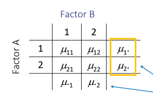
H01: 𝜇1. = 𝜇2. - main effect of factor A
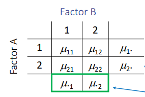
H02: 𝜇.1 = 𝜇.2 - main effect of factor B
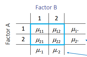
H03: (𝜇11 - 𝜇12) = (𝜇21 - 𝜇22) - interaction effect
Graph examples
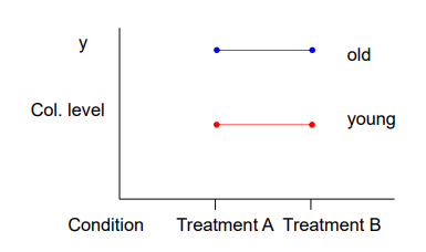
No main effect of treatment condition bc if we disregard age both conditions are equal (same/no slope)
Main effect of age bc old always score higher than young (position on Y axis)
No interaction bc lvl of col. is the same (lines are parallel)
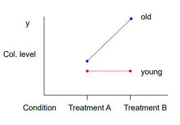
Main effect of treatment bc regardless of age, treatment A has lower lvl than gr. B
Main effect of age bc old > young
Yes interaction bc effect of treatment is different across age groups
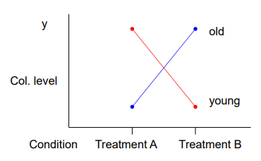
No main effect of treatment bc means of treat. A and B are equal
No age effect bc not one group consistently scores higher
Yes interaction
RQs
Main effect condition A: Is X the same across all lvl of A?
Main effect B: Is X the same for all lvl of B?
Interaction: Are the differences bet A the same for all of B?
Steps
Check assumptions (normal distribution, homogeneity of var.)
Check significance main effects and interaction (F-tests)
If interaction is significant → make interaction plot // If not sign → remove interaction and rerun mode (NOTE: never include interaction w/o main effects)
APA: The interaction bet. A and B was (not) found to be significant, F(df, df) = …, p = … . (After removal of the interaction term, both main effect were found significant)
Determine effect size (partial eta equared 𝜂2𝑝)
APA: The difference bet. A was significant, F(df, df) = …, p =…, 𝜂2𝑝 = …, indicating a … effect. The difference bet B was …
Do post-hoc comparisons
APA: Post-hoc tests revealed a significant difference bet. conditions C and D (p = …) and … . The difference bet. E and F was not significant (p = …)
Simple main effects - test dif. of 1 factor within other factor
APA: Simple main effects were significant for A1 (p = … ) and A2 (p = … ) // The mean scores for A1 differ significantly (p = … )
Report
APA: (interaction) The difference between private (M = 7.74, SD = 1.16) and public (M = 6.76, SD = 1.48) companies was significant, F(1, 76) = 13.13, p = .001, , 𝜂2𝑝 = .147, indicating a medium effect. The differences between the three experimental conditions (policies) were significant, F(2, 76) = 8.09, p = .001, 𝜂2𝑝 = .176, indicating a medium large effect.
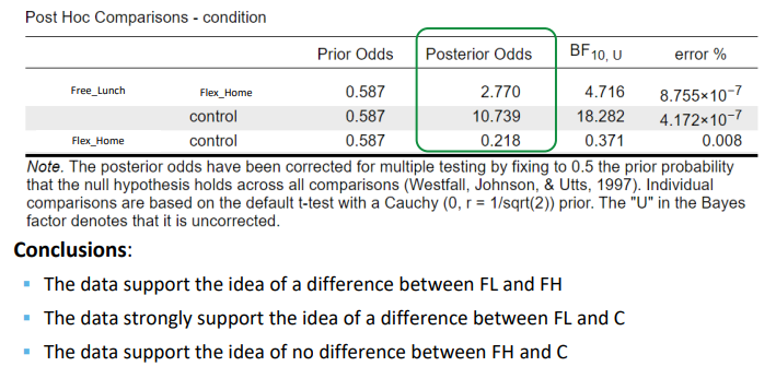
Post-hoc tests revealed a significant difference between the experimental conditions “Free Lunch but working from office” and “Flexible Home days” (p = .017) and between the experimental condition “Free Lunch but working form office” and the control group (p < .001). The difference between the experimental condition “Flexible Home days” and the control group was not significant (p =.975). Simple main effects were significant for both private (p = .018) and public (p = .021) companies.
Bayesian
Model 1 (null) condition + type
Model 2 - interaction
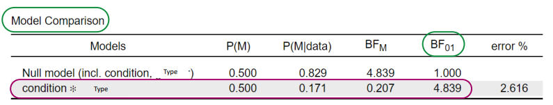
The model without the interaction effect has about 5 times more support in the data than the one with (BF01 = …)