MacroEcon Notes
Chapter 2: Thinking Like an Economist
1. Economists’ roles and tools
Scientists: Explain how the economy works using theories and evidence.
Policy advisers: Recommend what should be done.
Models: Simplified versions of reality, like graphs or equations.
Assumptions: Leave out extra details to make an issue easier to study.
2. Circular-flow model
Shows how households and firms exchange goods, resources, and money.
Households supply resources and buy goods and services.
Firms use resources to produce and sell goods and services.
In resource markets, firms pay households for labor, land, and capital.
In goods and services markets, households pay firms for products.
Remember: Money moves in the opposite direction from goods and resources. Capital means equipment and buildings used in production.
3. Production Possibilities Frontier (PPF)
Shows the combinations of two goods an economy can produce with its current resources and technology.
Inside the PPF: Possible, but inefficient—resources are underused.
On the PPF: Possible and productively efficient.
Outside the PPF: Currently impossible to produce.
Moving along the PPF means making more of one good by giving up some of the other.
4. Opportunity cost
What you give up to get something else.
Opportunity cost per unit = amount given up ÷ amount gained
Example: One computer requires 100 hours, while one ton of wheat requires 10 hours.
Cost of 1 computer = 10 tons of wheat.
Cost of 1 ton of wheat = 1/10 of a computer.
The PPF’s slope is negative, but opportunity cost is expressed as a positive amount.
5. Finding maximum production
Maximum output = total resources ÷ resources needed per unit
With 50,000 labor hours:
Computers: 50,000 ÷ 100 = 500 computers.
Wheat: 50,000 ÷ 10 = 5,000 tons of wheat.
These are separate maximums—you cannot produce both maximums at once.
6. PPF shape and growth
Straight PPF: Constant opportunity cost.
Bowed-out PPF: Increasing opportunity cost because resources are better suited to different tasks.
Outward shift: More productive capacity from additional resources or improved technology.
Moving from inside to the boundary: Better use of existing resources.
7. Microeconomics vs. macroeconomics
Microeconomics: Individual households, firms, and markets.
Macroeconomics: The whole economy, including inflation, unemployment, and growth.
8. Positive vs. normative statements
Positive: A claim that can be tested with evidence.
Example: “A higher price reduces the quantity purchased.”Normative: A judgment about what should happen.
Example: “Businesses should lower their prices.”
Positive does not mean true—it means testable.
Economists may disagree because they interpret evidence differently or have different values.
Chapter 3: Interdependence and the Gains from Trade
1. Key terms
Interdependence: Relying on others for goods and services.
Autarky: No trade; you consume only what you produce.
Exports: Goods sold to other countries.
Imports: Goods bought from other countries.
Specialization: Focusing production on particular goods.
2. Absolute vs. comparative advantage
Absolute advantage: Producing a good using fewer resources than another producer.
Comparative advantage: Producing a good at a lower opportunity cost.
Remember: Specialization and gains from trade are based on comparative advantage.
A country can have absolute advantage in both goods and still benefit from trade.
3. Calculating opportunity cost
When given hours needed per unit:
OC of A = hours for A ÷ hours for B
When given maximum outputs using the same resources:
OC of A = maximum output of B ÷ maximum output of A
Your answer tells you how much B you give up for one A.
4. U.S. and Japan example
The U.S. needs:
100 hours per computer.
10 hours per ton of wheat.
Therefore, one computer costs 10 tons of wheat.
Japan needs:
125 hours per computer.
25 hours per ton of wheat.
Therefore, one computer costs 5 tons of wheat.
The U.S. has absolute advantage in both because it uses fewer hours.
However:
Japan has comparative advantage in computers: 5 tons of wheat given up is less than 10.
The U.S. has comparative advantage in wheat: 1/10 of a computer given up is less than Japan’s 1/5.
Therefore, Japan exports computers and the U.S. exports wheat.
5. Mutually beneficial trade
For both sides to gain, the trading price must fall between their opportunity costs.
In this example, one computer should trade for more than 5 but less than 10 tons of wheat.
Suppose they trade one computer for 7 tons of wheat:
Japan receives 7 tons for a computer that costs it 5 tons to produce.
The U.S. pays 7 tons instead of sacrificing 10 tons to produce the computer itself.
6. Consumption after trade
Consumption = production + imports − exports
From the slides, the U.S. produces 160 computers and 3,400 tons of wheat. It imports 110 computers and exports 700 tons of wheat.
Computers consumed: 160 + 110 = 270.
Wheat consumed: 3,400 − 700 = 2,700 tons.
Trade allows consumption outside a country’s own PPF. It does not allow production outside it.
7. Does everyone gain from trade?
Trade can increase total output, product variety, and overall well-being.
However, some workers and businesses competing with imports may lose. An economy benefiting overall does not mean every person benefits.
Chapter 4 - The Market Forces of Supply and Demand
The Market - When supply meets demand
All the buyers and sellers of a particular good or service
Buyers as a group
Determine the demand for the product (Aggregate or market demand)
Sellers as a group
Determine the supply of the product (Aggregate or market supply)
The perfectly competitve market
Many buyers and many sellers of a good (Buyers and sellers are so numerous that no individual buyer or seller can affect the market price of the good)
Individual buyers and sellers are all price takers (they are aware of this)
The good is exactly the same (homogeneous good)
Demand
Quantity demanded, QD
- Amount of a good that buyers are willing and able to purchase at a given price
Law of Demand
Other things equal (income, price of other goods, etc.)
When the price of a good rises, the quantity demanded of the good falls
When the price falls, the quantity demanded rises
Aggregate Market Demand
Market Demand: sum of quantities demanded by all individuals of a good or service at any given price


Demand Curve Shifters
Linear demand curve, QD= a - bP
This shows how price affects quantity demanded, other things being equal
These ‘other things’ are non-price determinants of demand
Things that determine buyers’ demand for a good, other than the good’s price
Changes in them shift the D curve
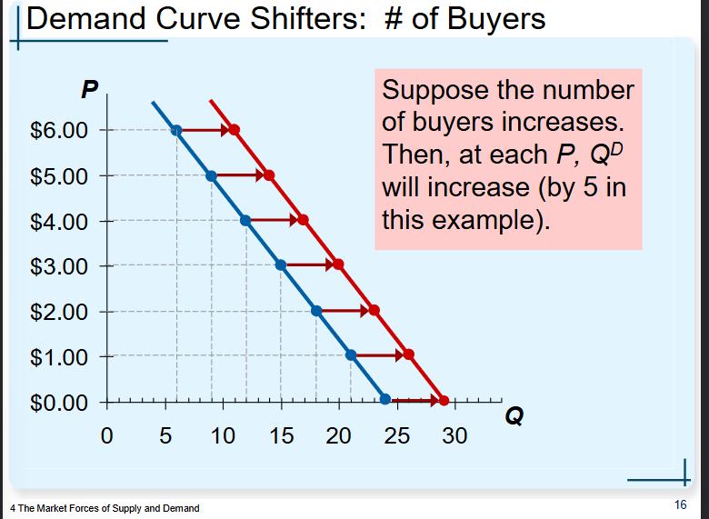
No. 1 - # of buyers
Increase in # of buyers(Increases quantity demanded at each price)
Shifts D curver to the right
Decrease in # of buyers(Decreases quantity demanded at each price)
Shifts D curve to the left
No. 2 - Income
Normal good, other things constant
An increase in income leads to a increase in demand —> Shifts D curve to the right
Inferior good, other things constant
An increase in income leads to a decrease in demand —> Shifts D curve to the left
No.3 - Prices of related goods
Two goods are substitutes if
an increase in the price of one leads to an increase in the demand for the other
Two goods are complements if
an increase in the price of one lead to an decrease in demand for the other (they’re consumed together)
No. 4 - Taste, preferences or trends
Anything that causes a shift in taste toward (or away from) a good will increase (or decrease) demand for that good at any given price and shift its D curve to the right (or left)
No. 5 - Expectations about the future
Expect an increase in income in the future => increase in current demand
Expect higher price in the future => increase in current demand

Supply
Quantity supplied, Qs
Amount of a good that sellers are willing and able to sell at a given price
Law of supply
Other things equal:
-When the price of a good rises, the quantity supplied of the good rises
-When the price falls, quantity supplied falls
Price and Quantity supplied moves in the same direction
Profit = Total Revenue (P x Q) - Total cost
When the ONLY change is that P increases:
Revenue increase
Profit per unit increases
more units means more profit
Supply schedule:
A table, shows the relationship between the price of a good and the quantity supplied at that price
Aggregate Market Supply
Sum of the supplies of all sellers of a good or service
Market supply curve: SUM of individual supply curves horizontally
To find the total quantity supplied at any given price, we add the individual quantities supplied at that price.
Supply Curve Shifters
The linear supply curve, Qs= c + dP
-Shows how price affects quantity supplied, other things being equal
These other things are non-price determinants of supply
-changes in them shift the entire S curve
Qs= c + dP
Qs= quantity supplied
P= Price of good
c= all factors affecting Qs other than P
+d = slope of the supply curve
No. 1 — Input prices
Supply is negatively related to prices of inputs (wages, prices of raw materials, prices of intermediate goods, etc.)
A fall in input prices, all else being the same, makes priduction more profirtable at each output price
Firms supply a larger quantity at each price
The S curve shifts to the right

No. 2 — Technology
Determines how much inputs are required to produce a unit of outputs
All else being the same, a cost-saving technological improvement has the same effect as a fall in input prices
shifts S curve to the right
No. 3 — Number of sellers
An increase in the number of sellers increases the quantity supplied at each price —> Shifts S curve to the right
No. 4 — Expectations about the future
Sellers may adjust current supply* when their expectations of future output prices change

Equailibrium: price has reached the level where quantity demanded equals quantity supplied: QD=Qs
Excess quantity supplied (surplus): quantity supplied is greater than quantity demanded
Excess quantity demanded (Shortage): quantity demanded is greater that quantity supplied
A shift in the D curve
Occurs when a non-price determinant of demand changes (like income or price of related goods)
A movement along a fixed D curve
Change in quantity, Occurs when P changes
A shift in the S curve
Occurs when a non-price determinant of supply changes (like technology or price of inputs)
Movement along a fixed S curve
Change in quantity supplied, Occurs when P changes

‘The Invisible Hand’ = decentralized allocation of resources: markets organize economic activity and coordinate actions by agents
In market economies prices adjust automatically to balance supply and demand
These equilibrium prices are the signals that guide economic decisions and thereby allocate scarce resources
Chapter 5 - Elasticity - measure of responsiveness of QDor Qs
To a change in one of their determinants
Price elasticity of demand
How much the quantity demanded of a good, QD, responds to a change in the price of that good, P
Loosely speaking, it measures the price- sensitivity of buyers’ demand
Midpoint
The midpoint is the number halfway between the start and the end value (always the same!!!)
In other words, the average of those two values
We will use the midpoint when computing percentage changes

Demand is elastic when quantity demanded is very responsive to changes in price (%∆quantity > %∆price)
Elastic when, Price elasticity of demand > 1
• Demand is inelastic ➔ Price elasticity of demand < 1
• Demand is unit elastic when ➔ Price elasticity of demand = 1
At the extremes
Demand is perfectly inelastic when Price elasticity of demand = 0, Demand curve is vertical
• Demand is perfectly elastic when Price elasticity of demand = infinity, Demand curve is horizontal
• The flatter the demand curve through a point => the greater the price elasticity of demand

Total Revenue = Price x Quantity
When D is elastic, a price increase causes revenue to fall
When D is inelastic, a price increase causes revenue to rise
In general, in order for a price increase to cause a decrease in total revenue, demand must be elastic
Quantity effect dominates = Increase in total revenue
Price effect dominates = decrease in total revenue
Price Elasticity of Supply
How much the quantity supplied of a good responds to a change in the price of that good
it measures sellers’ price-sensitivity or responsiveness to changes in output prices

Supply is unit elastic
Price elasticity of supply = 1
Supply is elastic
Price elasticity of supply >1
Supply is inelastic
Price elasticity of supply < 1
At extreme cases
Supply is perfectly inelastic, price of supply is 0
Supply is perfectly elastic, Price elasticity of supply is infinity
The flatter the supply curve => the greater the price elasticity of supply
Greater price elasticity of supply
The more easily sellers can change the quantity they produce or sell
Price elasticity of supply is greater in the long run than in the short run
When supply is inelastic, an increase price is more than on quantity
When supply is elastic, an increase in quantity is greater than price
Other Elasticities of Demand
Income elasticity of demand - How much the quantity demanded of a good respomds to a change in consumers’ income
Divided by the percentage change in income
Normal goods: income elasticity > 0
Inferior goods: income elasticity < 0
Cross-price elasticity of demand
How much the QD of one good responds to a change in the price of a related good
Divided by the percentage change in price of the related good
Substitutes: cross-price elasticity > 0
Complements: cross-price elasticity < 0
Chapter 10
Macroeconomics - Study of economy-wide phenomena and the factors that affect them
Inflation
Unemployment
Economic growth (=outward shifts of PPF)
Long run vs short run
Economic growth (long run trend) = growth of GDP in the long run
Business cycles (short run economic fluctuations) = short run ups (booms) and downs (busts) of GDP around its long run trend
High rate of growth of GDP
less unemployment and more inflation
Low or negative rate of growth of GDP
more unemployment and low or no inflation (perhaps even deflation)
Economic policy conundrum: Low or no growth and inflation = stagflation
Income and Expenditure
Gross Domestic Product (GDP)
Measures total income of everyone in the economy
Total production of output (goods and services) in the economy = national product
Also measures total expenditure on the economy’s output of goods and services
Income = Expenditure in a closed economy
For the economy as a whole
Because there is a seller and a buyer in every transaction:
Every dollar a buyer spends is a dollar of income for the seller
The circular-flow Diagram
Simple depiction of the macroeconomy
Illustrates GDP as production, as spending, and as income
Review:
Factors of production are inputs like labor, land, capital, and natural resources.
Factor payments are payments to the owners of the factors of production (wages, rent, interest, profit, dividends)
What The Diagram Omits
The government
Collects taxes, pays subsidies, buys goods and services, provides goods and services
The financial system
Matches savers’ supply of funds with borrowers’ demand for funds
The external or foreign sector
Trade goods and services, funds (in the form of financial assets), and currencies with the country’s residents
Formal Definition of GDP
…The market value of all final good and services produced within a country in a given period of time.
Goods are valued at their market prices so:
All goods and services (produced within a country) measured in the same unit. E.g., dollars in the U.S. Euros in the European Union
Goods and services that don’t have a market value (=price) are excluded:
Most items that are produced and consumed at home, such as housework you do for yourself, cooking, cleaning, caring for children, the sick, and the elderly.
Clean air, biodiversity, belonging
…the market value of all final goods and services produced within a country in a given period of time .
GDP includes all items produced in the economy and sold legally in markets.
GDP excludes activities within the underground (or shadow) economy:
Informal economy(domestic workers paid “off the books” unreported workers)
Items produced and sold illicity(drugs)
…the market value of all final goods and services proudced within a country in a given period of time
Goods can be
Final goods: intended for the end user
Intermediate goods: used as components or ingredients in the production of other goods
GDP only includes final goods, they already embody the value of all the intermediate goods used in their production.
the market value of all final goods and services proudced within a country in a given period of time.
GDP includes tangible goods (smart phones, mountain bikes, beer)
Intangible services (haircuts, concerts, cell phone service)
the market value of all final goods and services proudced within a country in a given period of time.
GDP measures the value if production that occurs within a country’s borders, whether done by its own citizens or by foreigners located there
the market value of all final goods and services proudced within a country in a given period of time.
GDP only measures goods and services produced during the current period
The current period is usually a year or a quarter (3 months).
GNP(Gross national product) - focus on the ownership of factors of prodution
The components of GDP
Recall: GDP is total spending.
4 expenditure components:
Consumption (C)
Investment (I)
Government Purchases (G)
Net Exports (NX)
These components must add up to GDP (denoted Y): Y ≡ C + I + G + NX
≡ - whatever changes right must change left.
Consumption, C
Total spending by households on goods and services
Note on housing costs:
Purchase of new housing NOT included in C
Rent payments are included in C:
For renters, C includes actual rent payments
For homeowners living in their own home: C includes the imputed rental value of the house
Investment, I
Total spending on goods that will be used in the future to produce more goods or services
Business capital: business structures, equipment, and intellectual property proudcts
Residential capital: landlord’s apartment building; a homeowner’s personal residence
Inventory accumulation: goods produced but not yet sold
In macroeconomics and national accounting (NIPA), ‘Investment’ does not mean the purchase of financial assets like stocks and bonds.
Government purchases (G)
All spending on goods and services purchased/produced by the government
At federal, state, and local levels
Excludes transfer payments
Such as social sercurity payments or unemployment insurance (UI) benefits
Not purchasing of goods and services
We want to avoid double counting
Net Exports (NX)
Net exports = exports - imports
Exports: foreign spending on the economy’s goods and services MUST BE ADDED
Imports: are the portions of C, I, and G that are spent on goods and services proudced abroad MUST BE SUBTRACTED
Real versus Nominal GDP
Nominal GDP
Values output using current prices
Not corrected for inflation
Real GDP
Values output using the prices of a base year (constant prices)
Is corrected for inflation
For the base year
Norminal GDP = Real GDP
Norminal GDP grows for 2 reasons
Prices are rising
the economy is producing a large quantity of goods
Real GDP only grows for one reasom
Prices stay the same (elimate inflation)
the econony only produces large quantity of goods
Real GDP would change if prices were constant (zero inflation) it reflects changes only in quantities.
The GDP Deflator
GDP deflator, for every period
A measure of overall level of prices

Measures the current level of prices relative to the level of prices in the base year
Economy’s annual inflation rate
Computes the percentage increase in the GDP deflator from one year to the next
Chapter 11
In the US, there are two primary measures of the prices paid by consumers for goods and services
Consumer Price Index (CPI), produced by the Bureau of Labor Statistics
Personal Consumption Expenditures price index (PCE or PCEI), prepared by the Bureau of Economic Analysis (BEA)
These two indexes are constructed differently and tend to behave differently over time
The Consumer price Index (CPI)
Measures the typical consumer’s cost of living
Measure of the overall cost of goods and sevices bought by the average consumer
Computed and reported every month by the BLS
It is the basis of cost-of-living adjustments (COLAs) in many contracts and in Social Security payments
Calculating the CPI
Compute the basket’s cost (monthly)
Use the prices to compute the total cost of the basket each month.
Choose a base year and compute the CPI
Cost of basket of goods and services in current year compared to cost of basket in base year

Compute the inflation rate
The percentage change in the CPI from the preceding period

Problems with the CPI
Substitution Bias
Over time, some prices rise faster than others.
Consumers substitute expenditure towards goods that become relatively cheaper, mitigating the effects of price increases on cost of living.
The CPI misses this substitution because it uses a fixed basket of goods.
Thus, the CPI tends to overstate increases in the cost of living.
Introduction of New Goods
The introduction of new goods increases variety, allows consumers to find products that more closely meet their needs.
In effect, dollars become more valuable
The CPI misses this effect because it uses a fixed basket of goods.
Thus, the CPI overstates increases in the cost of living.
Unmeasured Quality Change
Improvements in the quality of goods in the basket increase the value of each dollar.
The BLS tries to account for quality changes but probably misses some, as quality is hard to measure.
Thus, the CPI overstates increase in the cost of living.
Each of these problems causes the CPI to overstate cost of living increases.
Contrasting the CPI and GDP Deflator
Imported consumer goods:
Included in CPI
Excluded from GDP deflator
Capital goods:
Excluded from CPI
Included in GDP deflator (if produced domestically)
Intermediate goods
Excluded from both CPI and GDP deflator
The basket
CPI uses fixed basket
G&S actualized every ten years, weights and prices every month
GDP deflator uses ‘basket’ of currently produced goods & services
Does not need be actualized
This matters if different prices are changing by different amounts.
Correcting Variables for Inflation
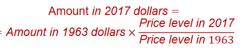
Comparing dollar figures from different times
Inflation makes it harder to compare dollar amounts from different times.
Example: the (federal) minimum wage
$1.25 in Dec 1963
$7.25 in Dec 2017
Minimum wage had more purchasing power in 1963
Indexation
A dollar amount is indexed for inflation if it is automatically corrected for inflation by law or in a contract.
The increase in CPI automatically determines:
The COLAs in many multi-year labor contracts, lease contracts.
Adjustments in Social Security payments and federal income tax brackets.
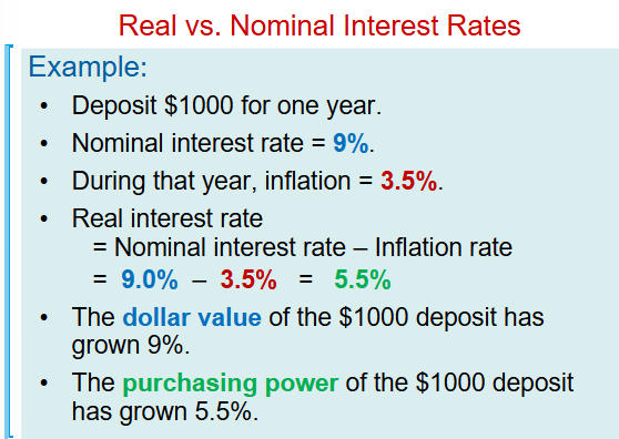
Real vs Nominal Interest Rates
The nominal interest rate:
Interest rate not corrected for inflation
Rate of growth in the dollar value of a deposit or debt
The real interest rate:
Corrected for inflation
Rate of growth in the purchasing power of a deposit or debt
Real interest rate = (nominal interest rate) – (inflation rate)
Chapter 13
Financial system
Group of institutions in the economy that help match the saving of one person with the investment of another
Financial instituions: Institutions through which savers can provide funds to borrowers
Directly through financial markets. Ex: NYSE
Indirectly through financial intermediaries, banks, mutual funds, pension funds (TIAA, Fidelity, etc.)
Financial Markets
Financial markets — Savers can directly provide funds to borrowers
The bond market (fixed income):
A bond is a certificate of indebtedness(IOU)
The stock market (variable income):
A stock (share, equity) is a claim to partial ownership in a firm
National Accounting Identities
Gross domestic product (GDP, formally Y)
Total income = Total expenditure
Y = C + I + G + NX (1)
Y = gross domestic product, GDP
C = consumption (households)
I = investment (mostly firms)
G = government purchases
NX = net exports
National saving (‘saving’), S
Total income in the econony that remains after paying for consumption of households and government purchases:
S = Y – C – G (2)
We use (2) to reformulate (1) as
(Y – C – G) – I = NX
When S>I country is net lender and NX>0
When S<I country is net borrower and NX<0
When S=I, country is neither, and NX = 0
Closed economy: EX = IM = 0, so that: Y = C + I + G (3)
National saving (‘saving’), S: Y – C – G = I (4)
It follows that, for a close economy: Saving (S) = Investment(I)
Accounting Identities
Indentity (4) can be rewritten as: (Y – T – C) + (T – G) = I
Where T are net taxes (total gov’t tax revenue minus transfer payments)
Private saving, (Y - T) - C
Income that households have left after paying for (net) taxes (=disposable income) and consumption
Public saving, T-G
Net tax revenue that the government has left after paying for its spending
The government can exhibit:
Budget surplus: T - G > 0
Excess of tax revenue over government spending = public saving = T - G > 0
Budget deficit: T - G < 0
Shortfall of tax revenue from government spending = -public saving = T - G < 0, which can also be expressed as G - T > 0
The Meaning of Saving and Investment
What private saving is:
Income remaining after households pay their (net) taxes and pay for consumption.
Some of the things households do with saving:
Buy corporate bonds or equities
Purchase a certificate of deposit at the bank
Buy shares of a mutual fund
Let accumulate in saving or checking accounts
What investment is
the purchase or making of new capital
Examples of investment:
General Motors spends $250 million to build a new factory in Flint, Michigan
You buy $5000 worth of computer equipment for your business
Your parents spend $300,000 to have a new house built.
Investment is NOT the purchase of stock and bonds!
The Market for Loanable Funds
A supply-demand model of the financial system
Helps us understand:
How the financial system coordinates saving & investment
How government policies and other factors affect
Saving(=supply of loanable funds),
Investment(=demand of loanable funds), and
the interest rate (= price of loanable funds).
Simplifying assumptions
Only one financial market
All savers (households) deposit their saving in this market.
All borrowers (mostly firms) take out loans from the market.
There is one interest rate, which is bothe the return to saving and the cost of borrowing.
The supply of loanable funds comes from:
Private saving
Households with extra income can loan it out and earn interest.
Public saving
If positive, adds to national saving and the supply of loanable funds
If negative, reduces national saving and the supply of loanable funds.
The demand for loanable funds comes from investment:
Firms borrow the funds they need to pay for new equipment, factories, R&D, etc.
Households borrow the funds they need to purchase new houses.
Budget Deficits, Crowding Out, and Long-Run Growth
In our analysis:
Increase in budget deficit causes fall in private investment (investment by firms and households)
The government borrows to finance its deficit, leaving less funds available for investment by the private sector: crowding out
Investment is important for long-run economic growth
If budget deficits do not finance government investment, they reduce the economy’s growth rate and future standard of living.
The U.S. Government Debt
The government finances deficits by borrowing (i.e., selling government bonds).
Persistent deficits lead to a rising government debt.
The ratio of government debt to GDP
Useful measure of the government’s indebtedness relative to its ability to raise tax revenue.
Historically, the debt-GDP ratio rises during wartime and falls during peacetime—until the early 1980s (the ‘Reagan years’)
Conclusion
Competitive markets are usually a good way to organize economic activity
If financial markets are governed by the forces of supply and demand
Allocate the economy’s scarce L.F. to their most efficient uses (=highest return uses).
Link the present to the future
Savers: convert current income into future purchasing power
Borrowers: acquire capital to produce goods and services in the future
Summary
The U.S. financial system is made up of many types of financial institutions, like the stock and bond markets, banks, and mutual funds.
National saving equals private saving plus public saving.
In a closed economy, national saving equals investment. This happens in the financial system.
The supply of loanable funds comes from saving. The demand for funds comes from investment. The interest rate adjusts to balance supply and demand in the loanable funds market.
A government budget deficit is negative public saving, so it reduces national saving, the supply of funds available to finance private investment.
When a budget deficit crowds out private investment, it may reduce the growth of productivity and GDP.