Analyzing Data through Linearization and Composition

Semi-Log Plots and Linearization

In science and mathematics, data often spans several orders of magnitude, or follows a non-linear growth pattern. A semi-log plot is a specialized graphing technique used to visualize exponential functions as straight lines. This process is often called linearization.

The Concept of Linearization

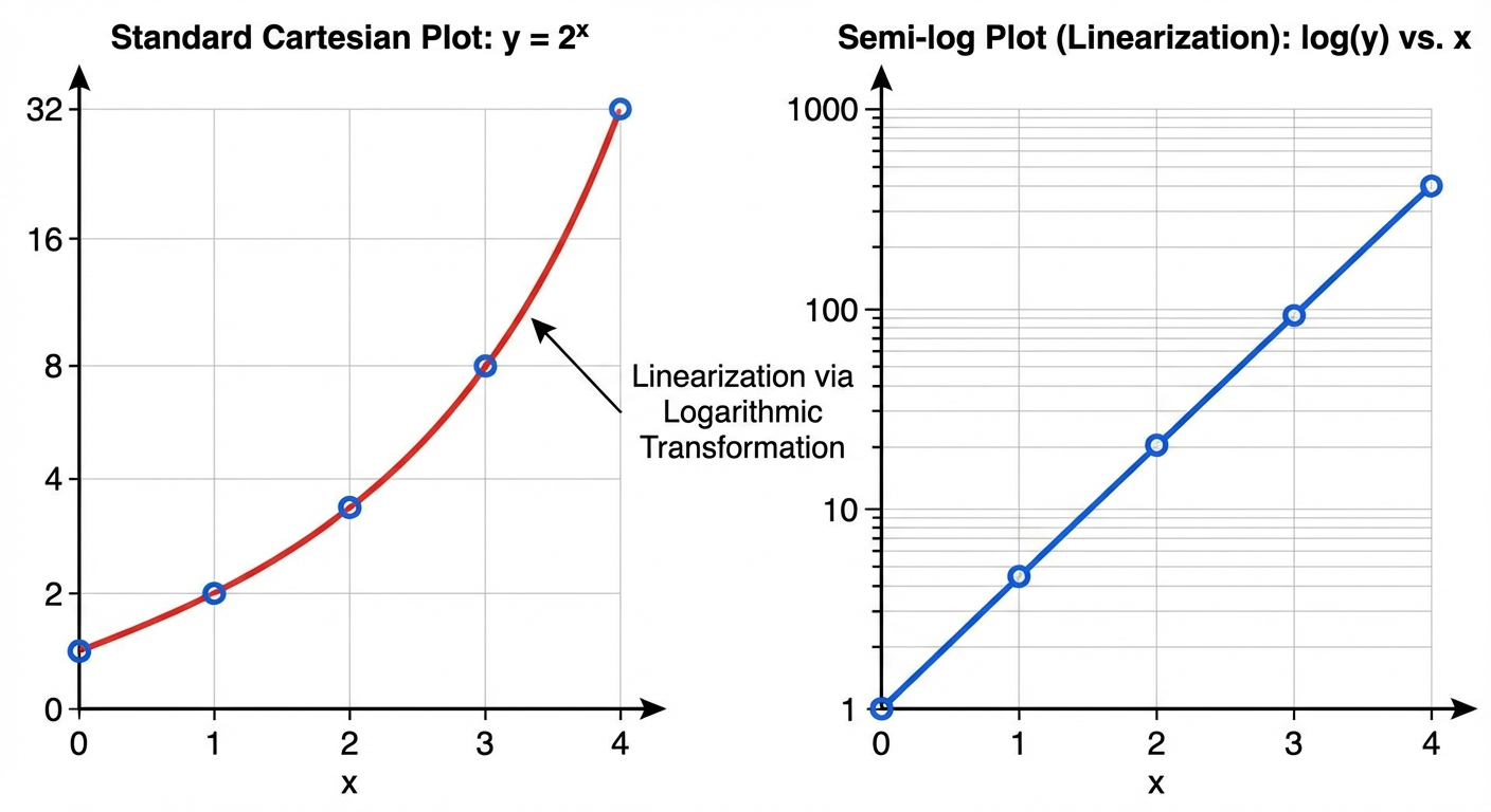
When you graph an exponential function like $y = ab^x$ on a standard Cartesian coordinate system (linear scales on both axes), the result is a curve. Determining specific parameters (like $a$ and $b$) just by looking at a curve is difficult.

However, if we transform the output values using logarithms, the exponential relationship transforms into a linear one. This allows us to use linear regression tools or simple slope calculations to model the data.

• Standard Plot: $x$ vs. $y$ produces a curve.
• Semi-Log Plot: $x$ vs. $\log(y)$ (or $\ln(y)$) produces a straight line.

Deriving the Linear Form

To understand why this works, we apply properties of logarithms to the standard exponential equation.

Starting with the exponential model:
$y = a \cdot b^x$

Take the logarithm (natural or base 10) of both sides:
$\ln(y) = \ln(a \cdot b^x)$

Apply the product rule of logarithms ($\ln(mn) = \ln m + \ln n$):
$\ln(y) = \ln(a) + \ln(b^x)$

Apply the power rule of logarithms ($\ln(x^p) = p \ln x$):
$\ln(y) = \ln(a) + x \cdot \ln(b)$

Rearrange to look like the slope-intercept form ($Y = mx + k$):
$\underbrace{\ln(y)}<em>{Y} = \underbrace{(\ln b)}</em>{m} \cdot x + \underbrace{\ln(a)}_{k}$

In this linearized equation:

• The input represents $x$.
• The output represents $\ln(y)$ (the log of the original data).
• The slope ($m$) represents $\ln(b)$ (the log of the growth factor).
• The y-intercept ($k$) represents $\ln(a)$ (the log of the initial value).

Analyzing Data from Semi-Log Plots

If you are given a data set or a graph where the $y$-axis is on a logarithmic scale and the data forms a line, you can conclude the underlying relationship is exponential.

Steps to Find the Exponential Equation:

1. Calculate the Linear Equation: Find the slope ($m$) and y-intercept ($k$) of the line using the points $(x<em>1, \log y</em>1)$ and $(x<em>2, \log y</em>2)$.
2. Solve for the Base ($b$): Since $m = \ln b$ (or $\log b$), use the inverse log property:
   $b = e^m \quad \text{(if natural log is used)}$
   $b = 10^m \quad \text{(if common log is used)}$
3. Solve for the Coefficient ($a$): Since $k = \ln a$:
   $a = e^k$

Modeling with Exponential and Logarithmic Functions

Mathematical modeling involves choosing a function that behaves similarly to a real-world phenomenon. In AP Precalculus, you must distinguish between scenarios that require exponential models versus those that require logarithmic models.

Determining the Model Type

Concavity and Growth Rates

When looking at a scatterplot or data table, the concavity and rate of change help identify the function.

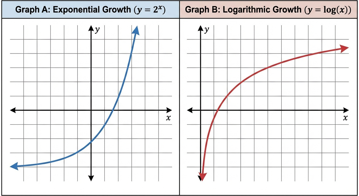
• Exponential Growth ($b > 1$): Increasing and concave up. The rate of change increases rapidly as $x$ increases.
• Logarithmic Growth ($b > 0$): Increasing and concave down. The rate of change decreases (slows down) as $x$ increases, but the function theoretically grows without bound.

Worked Example: Modeling from Data

Problem: A researcher collects the following data:

Solution:

1. Check for Equal Intervals: The input $t$ increases by 2 every step (arithmetic).
2. Check Ratios: Calculate the ratio of consecutive outputs:
   $140 / 50 = 2.8$
   $392 / 140 = 2.8$
3. Conclusion: Since the ratios are constant, this is an exponential model.
4. Form: $V(t) = a \cdot b^t$.
   • At $t=0$, $V(0) = 50$, so $a = 50$.
   • Since the interval is 2 hours, the growth over 2 hours is $2.8$. So $b^2 = 2.8 \implies b = \sqrt{2.8} \approx 1.673$.
   • Model: $V(t) = 50(1.673)^t$.

Composition of Exponential and Logarithmic Functions

Function composition involves substituting one function into another, denoted as $f(g(x))$. When combining exponential and logarithmic functions, compositions often utilize inverse properties to simplify expressions or model complex behaviors.

Inverse Properties

Because $f(x) = b^x$ and $g(x) = \log_b x$ are inverse functions, their compositions cancel out, leaving the argument unchanged (provided the domain is valid).

1. $\log_b(b^x) = x$
2. $b^{\log_b x} = x$ (for $x > 0$)

Modeling with Composition

Composition is frequently used to transform variables or combine rates.

Example: Atmospheric Pressure
Let input $h$ be altitude in kilometers. The pressure $P$ in millibars decreases exponentially: $P(h) = 1000(0.88)^h$.
Suppose altitude $h$ depends on time $t$ effectively linearly as a weather balloon rises: $h(t) = 0.5t$.

The pressure with respect to time is a composition $P(h(t))$:
$P(h(t)) = 1000(0.88)^{0.5t} = 1000(0.88^{0.5})^t \approx 1000(0.938)^t$

Domain and Range of Compositions

When finding the domain of $f(g(x))$:

1. $x$ must be in the domain of the inner function $g(x)$.
2. The output $g(x)$ must be in the domain of the outer function $f(x)$.

Example: Let $f(x) = \log(x)$ and $g(x) = 4 - x^2$.
Find the domain of $f(g(x)) = \log(4 - x^2)$.

• Constraint: The argument of the log must be positive.
• $4 - x^2 > 0$
• $-x^2 > -4 \implies x^2 < 4$
• Domain: $(-2, 2)$.

Common Mistakes & Pitfalls

1. Confusing Plot Axes for Linearization:

   • Mistake: Thinking that plotting $\log x$ vs. $\log y$ linearizes an exponential function.
   • Correction: $\log x$ vs. $\log y$ linearizes a Power Function ($y=ax^p$). For Exponential Functions ($y=ab^x$), you must plot $x$ vs. $\log y$ (semi-log).

2. Misinterpreting the Slope on a Semi-Log Plot:

   • Mistake: Assuming the measured slope of the linearized data is the base $b$.
   • Correction: The slope of the line is $\ln(b)$ (or $\log(b)$ depending on the base used). You must exponentiate the slope to find the actual growth factor: $b = e^{slope}$.

3. Domain Violations in Composition:

   • Mistake: Canceling out functions without checking constraints, e.g., claiming $e^{\ln(-5)} = -5$.
   • Correction: The domain of $\ln(x)$ is $(0, \infty)$. You cannot take the log of a negative number, so the expression is undefined, not $-5$.