day 5 part 1 Economics: Demand and Marginal Benefit

Context and Objectives * The session focuses on technical intricacies of the demand-supply model. * The goal is to move beyond surface-level understanding to develop an intuitive feel for how the model applies to real-life applications.

Salary Statistics in America * The average entry-level teacher salary is approximately $38,600$ per year. * In contrast, the average entry-level financial analyst earns approximately $74,101$ per year.
The Paradox of Importance * There have been significant public protests and strikes across the United States, documented by sources like Time Magazine, regarding teacher compensation. * Teachers are arguably more fundamental to society than financial analysts, as analysts, engineers, and other professionals require high-quality education and inspiration from teachers (e.g., math teachers) to enter their respective fields. * Despite their foundational importance, teachers are paid significantly less than financial analysts.

Utility vs. Price * Water is essential for human survival; death occurs within approximately three days without hydration ("drying out" or dying). * Diamonds serve no biological or survival purpose; a person can live a perfectly healthy life without ever owning a diamond.
Market Valuation Gap * A standard bottle of water costs approximately just below $1.50$ on average. * A single diamond can be valued at several millions of dollars. * This paradox invites an investigation into why "useless" products command high prices while essential ones do not.

Definition of Marginal Benefit ( $MB$ ) * Marginal Benefit is the additional benefit a consumer receives from consuming exactly one more unit of a good or service. * It is also referred to as the Expected Additional Benefit ( $EAB$ ).
Application Example: Ron Weasley and Butterbeer * In the context of Harry Potter, Ronald Weasley's marginal benefit from butterbeer is the specific satisfaction gained from drinking one additional cup/bottle.
Principle of Diminishing Marginal Benefit * This is the fundamental concept driving the downward slope of the demand curve. * The principle states that each additional unit of a good consumed provides less benefit than the previous unit. * Practical example: Professor Jacob Clifford's experience drinking a gallon of milk—initial consumption may be satisfying, but every subsequent cup yields decreasing satisfaction until sickness occurs. * Pizza consumption example: The first slice of pizza (especially after a long day of physical activity like moving boxes) provides high happiness/satisfaction. However, as one continues to eat, the additional satisfaction from each subsequent slice decreases.

Logic of the Buyer * Buyers want less of what they already have in abundance because the additional satisfaction from more units is lower. * Crucially, because additional benefit falls, the price a buyer is willing to pay for each additional unit also falls.
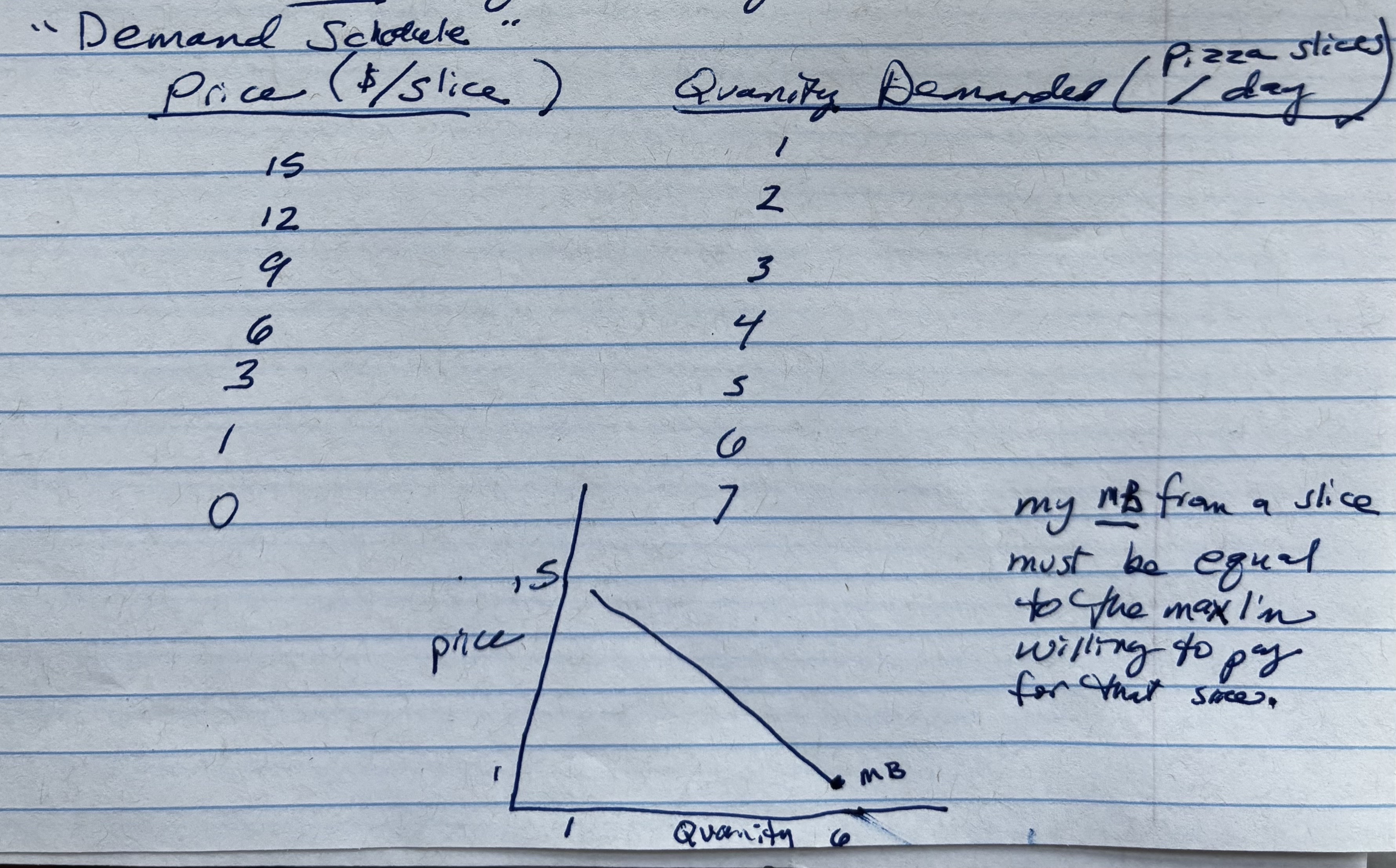
Individual Demand Schedule Example (Pizza) * 1st Slice: Marginal Benefit is high; Willingness to Pay ( $WTP$ ) is $15$ . * 2nd Slice: Following diminishing marginal benefit, the value is lower; $WTP$ is $12$ . * 3rd Slice: Marginal Benefit decreases further; $WTP$ is $9$ . * The "Demand Schedule" is the formal list containing the quantities demanded at various price points.

Coordinates and Plotting * Vertical Axis (Y): Price ( $dollars/slice$ ). * Horizontal Axis (X): Quantity Demanded ( $slices/day$ ). * Specific data points from the example include: * $\text{Price } 15 \rightarrow \text{Quantity } 1$ * $\text{Price } 6 \rightarrow \text{Quantity } 4$ * $\text{Price } 1 \rightarrow \text{Quantity } 6$
Optimization and Economizing Behavior * To optimize, a consumer matches their Marginal Benefit ( $MB$ ) to the maximum price they are willing to pay. * If a consumer pays more than their $MB$ , they violate the rule of expected additional benefit: $\text{Expected Additional Benefit (EAB)} \geq \text{Expected Additional Cost (EAC)}$ . Paying more than the benefit results in EAC > EAB.
Key Geometric Insight * The height of the demand curve at any specific quantity measures the Marginal Benefit ( $MB$ ) for that particular unit.

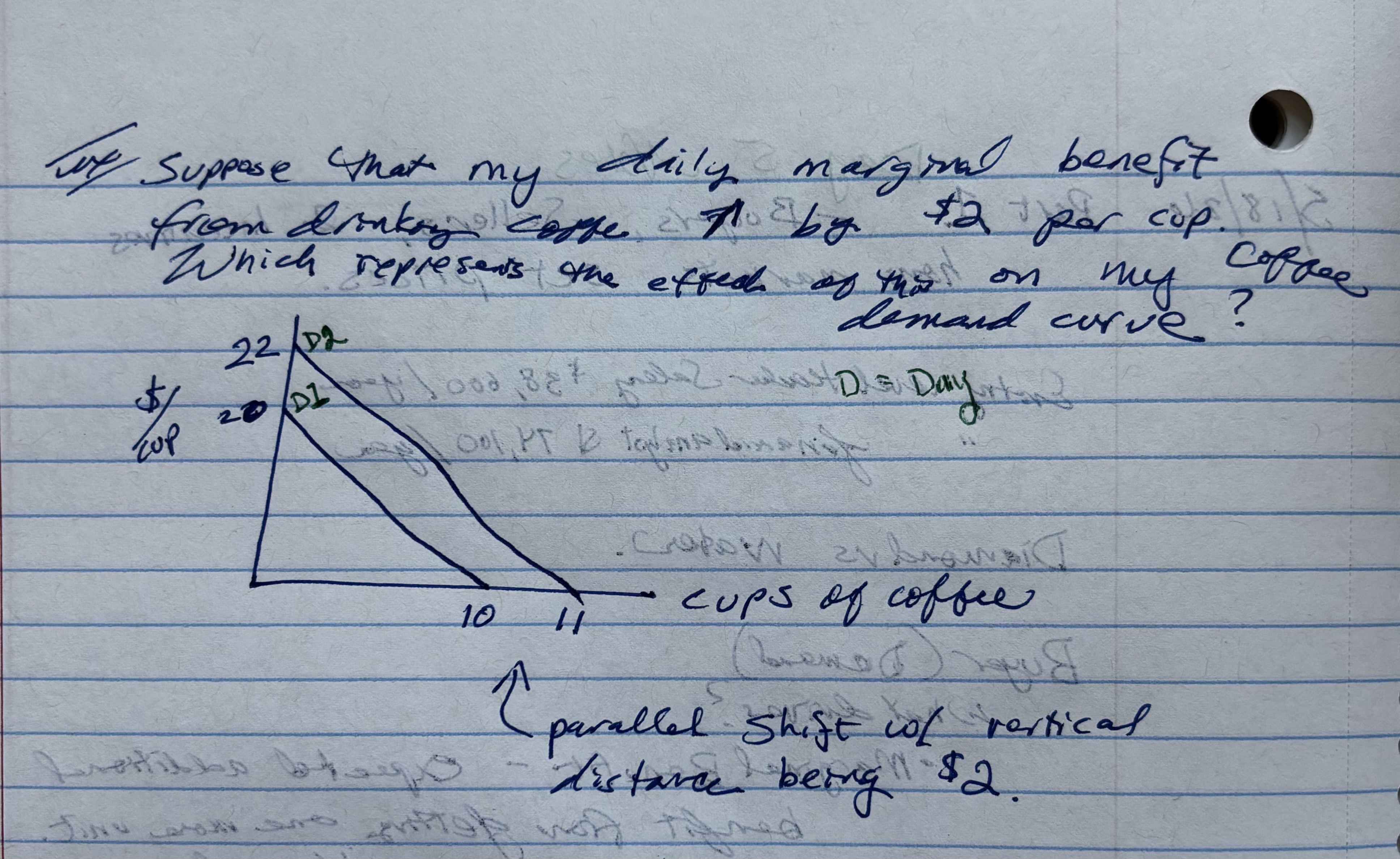
Scenario: Marginal Benefit Increase * Assume a daily marginal benefit for coffee increases by $2$ per cup across all quantities.
Initial Demand Conditions ( $D_1$ ) * Vertical Intercept: $20$ * Horizontal Intercept: $10$
Calculating the New Demand Curve * At zero cups, the original $MB$ was $20$ . With the increase, the new vertical intercept is $20 + 2 = 22$ . * At an arbitrary quantity (e.g., $5$ cups), if the old price was $10$ , the new price is $10 + 2 = 12$ . * At $10$ cups, the old $MB$ was $0$ (the horizontal intercept). The new $MB$ is now $0 + 2 = 2$ .
Visualizing the Shift * The new demand curve represents a parallel shift of the old curve. * The vertical distance between the old curve ( $D_1$ ) and the new curve is exactly equal to the change in marginal benefit ( $2$ ) at every point.