Consumption, Saving, and Investment Study Notes
Consumption, Saving, and Investment
Desired Consumption and Saving
Introduction of the concept of desired consumption (Cᵈ):
The aggregate quantity of goods and services that households want to consume based on available income and other influencing factors (e.g., interest rates).
Saving = income that is not consumed.
Desired consumption is what we may hypothetically consume for any given income and other factors (think about labour demand and labour supply).
Actual consumption is what we actually observe from data.
The Consumption and Saving Decision
Decision-Making Process
Individuals face a trade-off between current consumption and future consumption:
A trade-off: current consumption and future consumption
A person saves because she believes her future consumption could be lower (e.g., unemployment, health issues, accidents).
General tendency: People aim to smooth consumption over time, avoiding large fluctuations.
Impacts of Income Changes
Extra Income:
1. Extra Income – What Happens When Someone Earns More
If a person receives some extra income (like a raise, bonus, or increase in wealth), they will usually:
Spend some of it on goods and services (consume more)
Save some of it for the future
They typically don’t spend all of the extra money because people like to smooth their consumption over time — meaning they prefer to spread their spending evenly throughout their life rather than all at once.
2. Marginal Propensity to Consume (MPC)
The Marginal Propensity to Consume (MPC) measures how much of each extra dollar earned is spent on consumption.
Formula:
MPC = (Change in Consumption) ÷ (Change in Income)Example:
If MPC = 0.4 and your income increases by $100, you will spend $40 and save $60.
This shows that only part of the additional income is used for consumption, while the rest is saved.3. Why 0 < MPC < 1
MPC can’t be 0 because people usually spend some of their new income.
MPC can’t be 1 because people also save some of it.
Therefore, MPC always lies between 0 and 1.
This means both consumption and saving increase when income rises.
4. If Future Income Is Expected to Increase
If people expect their income to rise in the future, they will start spending more now, even before their income increases.
This happens because they feel wealthier and want to maintain a consistent lifestyle.Current consumption increases
Current saving decreases
5. Key Idea – Consumption Smoothing
People prefer to keep their consumption relatively steady over time.
When their income changes (now or in the future), they adjust their consumption and saving to maintain a stable lifestyle — not spending too much in one period or too little in another.
Interest rate
Real interest rate determines the benefit of saving (or the cost of not saving).
If you consumed one less dollar today and saved it, you could consume 1+r more dollars tomorrow.
Alternativley, you could consume one more dollar today, at the cost of consuming 1+r fewer dollars tomorrow.
The real interest rate determines the relative price of current consumption and future consumption.
Substitution effect:
This is about how the relative “price” of consuming today versus saving for tomorrow changes.
When the interest rate increases, saving becomes more rewarding — you earn more in the future for every dollar you save today.
Because of that, spending money today (consuming) now has a higher “opportunity cost,” since you give up more future income by not saving.
So people tend to consume less now and save more.
Income effect:
This focuses on how your overall wealth changes.
When the interest rate goes up, your future income increases (because your savings will grow faster).
You might then feel richer, and since you’re richer, you may want to consume more today even though saving pays more.
Overall Effect
These two effects work in opposite directions:
Substitution effect → save more, consume less today.
Income effect → consume more today (since you’re richer).
Because they pull in opposite ways, the overall effect is ambiguous — it depends on which effect is stronger.
Usually, the substitution effect is stronger, meaning: Higher real interest rates → less current consumption and more saving.
Taxes
Typically, saving comes from after-tax income.
Interest income is also subject to taxes.
r = (1 - t)i - πᵉ
That equation shows how taxes and inflation affect the real (after-tax) interest rate that a person actually earns from saving.
r = real after-tax interest rate (the true return on saving, adjusted for both taxes and inflation)
t = tax rate on interest income
i = nominal interest rate (the interest rate before accounting for taxes or inflation)
πᵉ = expected inflation rate
To encourage saving, the government can:
Allow part of the saving to be tax-deductable (RRSP)
Allow part of the interest income to be tax-exempt (TFSA)
Fiscal Policy
Suppose the government decides to increase its expenditure (G)
Higher (G) can be financed in two ways:
Option 1: Increasing Current Taxes
By increasing current taxes, this lowers Cᵈ but by less than the increase in (G). Higher taxes reduce people’s disposable income, which lowers desired consumption (Cᵈ).
However, Cᵈ decreases by less than the increase in G, because households typically reduce some consumption but not by the full amount of the tax increase (they may use some savings to maintain spending).
As a result, overall spending (Cᵈ + G) increases slightly.
Option 2: Borrowing Now and Raising Taxes Later
The government can borrow money now and promise to repay it with higher taxes in the future.
Borrowing allows G to increase immediately, but people know taxes will rise later to repay the debt.
This expectation causes a small decrease in current consumption (Cᵈ) because households anticipate lower future disposable income.
Still, Cᵈ falls by less than the rise in G, so total spending today increases.
By borrowing today and increasing future taxes. This lowers Cᵈ but by less and the increase in G. This is because:
When the government borrows money to increase spending (G), it does not raise taxes immediately. Instead, it plans to repay that borrowed money later by increasing taxes in the future.
Because people understand that higher taxes are coming later, they expect their future disposable income to decrease. This expectation causes them to slightly reduce current consumption (Cᵈ) in order to save more and prepare for those future taxes.
However, the decrease in Cᵈ is smaller than the increase in G, because:
The tax increase hasn’t happened yet.
Some households may not fully adjust their spending for future taxes.
People tend to smooth their consumption over time, spreading out the impact of income changes.
As a result, while government spending rises, private consumption only falls slightly, leading to an overall increase in total demand (Cᵈ + G).
Remember that S = Y – C – G + NFP
Desired saving: Sᵈ = Y – Cᵈ – G if NFP = 0
Desired national saving Sᵈ will decrease whether G is financed through taxes or borrowing because:
When the government increases its spending (G), total desired national saving (Sᵈ) decreases no matter how that spending is financed — through higher taxes or borrowing.
Here’s why:
If G is financed by higher current taxes:
Households have less disposable income, so they consume less (Cᵈ decreases).
However, the reduction in consumption is smaller than the increase in government spending, meaning total saving falls.If G is financed by borrowing (future taxes):
People know taxes will rise in the future to repay the debt, so they slightly reduce current consumption now.
But again, this decrease in Cᵈ is smaller than the increase in G, so desired national saving still falls.
In both cases, the government’s higher spending uses up part of the economy’s total resources. Since households’ reduction in consumption does not fully offset this, less is left over for saving.
Marginal Propensity to Consume (MPC):
What Is the Cost of Having One More Unit of Capital?
The user cost of capital per year is made up of two parts:
The interest cost per year, and
The depreciation cost per year.
Formula: uc = r × pₖ + d × pₖ
where:
r = real interest rate
pₖ = real price of capital
d = depreciation rate
Example:
Suppose a type of machine costs $100 per unit, the real interest rate (r) is 4%, and the depreciation rate (d) is 10%.
Then:
uc = 4% × $100 + 10% × $100 = $14 per yearWhy Is It Less Than the Purchase Cost ($100)?
The user cost of $14 per year represents the annual cost of using the machine, not the cost to buy it. The $100 purchase price is a one-time investment, while $14 reflects how much it costs to own and use that machine each year due to interest and depreciation.
Will There Be an Interest Cost if the Firm Is Not Borrowing?
Yes, there will still be an interest cost, even if the firm is not borrowing. This is because the interest represents an opportunity cost — the return the firm gives up by investing its money in the machine instead of putting it elsewhere (for example, in the bank or in another investment).
Expected Future Income:
An increase in expected future income drives down current saving and elevates consumption levels due to similar consumption-smoothing behaviors.
Understanding Investment
Definition and Implications
Investment refers to the purchase or construction of capital goods.
The investment decision resembles that of consumption-saving:
More investment today → lower profit for firm owners today
More investment today → potentially higher output and higher income for firm owners in the future.
Marginal Product of Capital ( ):
The expected future marginal product of capital: the expected future benefit of increasing investment.
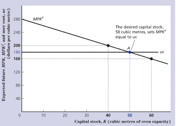
Desired Capital Stock
The desired capital stock is the capital stock where MPKᶠ = uc
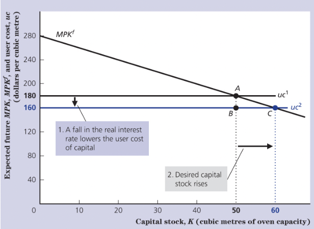
Impact of Interest Rate and Technological Changes
A decrease in real interest rates leads to a decreased user cost ; implications for desired capital stock.
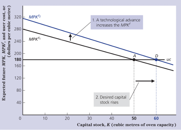
A technological improvement makes machines, tools, and equipment more productive.
That means the same amount of capital now produces more output, so MPKᶠ increases.
As a result, firms want to invest in more capital, since each unit of capital now gives a higher return.
Therefore, desired capital stock rises.
Taxation on Revenue
Taxation on Revenue
Firms must pay a fraction (τ) of the return from capital as tax to the government.
In other words, instead of getting MPKᶠ, firms receive (1 – τ)MPKᶠ after taxes.
Or, MPKᶠ = uc / (1 – τ)
We also call uc / (1 – τ) the tax-adjusted user cost of capital.
If τ increases:
(1 – τ) gets smaller.
uc / (1 – τ) gets larger → the cost of using capital (after taxes) rises.
Firms now need a higher MPKᶠ to justify investing.
Since MPKᶠ falls as you add more capital, the firm will choose to have less capital.
Investment and Capital Dynamics
Relationship and Definitions
Capital increase derives from net investment, defined as:
Increase in capital = investment (new capital) - depreciation of existing capital
We refer to investment - depreciation as net investment
Identification of desired investment:
Let K* be the desired capital stock, and let Kₜ denote the current capital stock.
Desired investment:
Iᵈ = K* – (Kₜ – dKₜ)Numerical Example of Desired Investment
Example:
Suppose the tax-adjusted user cost of capital is equal to 4, while the expected marginal product of capital is given by:
8 – 0.1KHere, K represents the capital input. Suppose the current capital stock is 30 and the depreciation rate is 10%. What is the desired investment?
Step 1: Use uc = MPKᶠ to calculate desired capital
4 = 8 – 0.1K → K* = 40
Step 2: Calculate desired investment
Iᵈ = 40 – (30 – 10% × 30) = 13
✅ Explanation:
First, we find the desired capital stock (K*) by setting the marginal product of capital (MPKᶠ) equal to the user cost of capital (uc).
Then, we calculate desired investment (Iᵈ) using the formula:
Iᵈ = K* – (Kₜ – dKₜ)Plugging in the numbers gives Iᵈ = 13, meaning the firm should invest 13 units to reach its desired level of capital.
Goods Market Equilibrium
Goods Market Equilibrium
The goods market equilibrium happens when desired saving (Sᵈ) equals desired investment (Iᵈ).
We start with these relationships:
Sᵈ = Y – Cᵈ – G
(Saving is what’s left from total income (Y) after consumption (Cᵈ) and government spending (G).)We also know that total output (income) is equal to total spending:
Y = Cᵈ + Iᵈ + G
Rearranging this gives:
Iᵈ = Y – Cᵈ – G
Notice that this is the same as Sᵈ, which means:
Sᵈ = Iᵈ
What this means:
This equality represents the goods market equilibrium, where total output (Y) is fully used for consumption, investment, and government spending.
Individuals decide how much to save (Sᵈ).
Firms decide how much to invest (Iᵈ).
So how does the market ensure that Sᵈ = Iᵈ?
The real interest rate adjusts to bring the market into balance.
If saving exceeds investment, there is excess supply of funds, which causes the real interest rate to fall.
If investment exceeds saving, there is excess demand for funds, which causes the real interest rate to rise.
Eventually, the interest rate settles at a level where desired saving equals desired investment, creating goods market equilibrium.
We call it goods market equilibrium
Goods market equilibrium means that the total amount people want to save (Sᵈ) equals the total amount firms want to invest (Iᵈ).
If people save more than firms want to invest, there’s extra money sitting around → not all goods produced are being bought → output falls.
If firms want to invest more than people are saving, there isn’t enough money to finance that → interest rates rise to encourage more saving.
Who determines what?
Households decide how much to save (based on income, interest rates, etc.).
Firms decide how much to invest (based on profitability, interest rates, etc.).
How does the market ensure Sᵈ = Iᵈ?
The interest rate (r) adjusts to bring the two into balance:
If Sᵈ > Iᵈ, interest rates fall → people save less, firms invest more.
If Sᵈ < Iᵈ, interest rates rise → people save more, firms invest less.
Eventually, they meet at the point where desired saving = desired investment, achieving goods market equilibrium.
Achieving Equilibrium
The goal:
We want desired saving (Sᵈ) to equal desired investment (Iᵈ) — that’s when the goods market is in equilibrium.
1. What links saving and investment?
The key factor that affects both is the real interest rate (r).
It’s the “price” of borrowing and lending money:
Households decide how much to save depending on r.
Firms decide how much to invest depending on r.
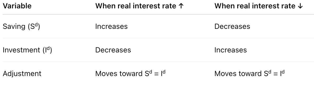
2. Saving (Sᵈ) increases when the real interest rate rises
When r increases, people earn more return on savings.
Consuming now becomes more expensive (substitution effect), so people save more and consume less.
Therefore, the supply of saving (Sᵈ) increases with higher interest rates.
3. Investment (Iᵈ) decreases when the real interest rate rises
For firms, the user cost of capital (cost of borrowing or using funds for investment) goes up when r increases.
That makes it less profitable to invest in new capital (machines, equipment, etc.).
So, investment (Iᵈ) decreases as interest rates rise.
4. How equilibrium is achieved
If r is too low → firms want to invest a lot, but households don’t save enough → shortage of funds → interest rate rises.
If r is too high → households save a lot, but firms don’t want to borrow → excess savings → interest rate falls.
Eventually, the real interest rate adjusts to the point where Sᵈ = Iᵈ
Numerical Examples and Consequences
Application of Changes in G
Suppose Y = 300 and G = 50. Desired consumption and desired investment are given by: Cᵈ = 200 – 100r + 0.1Y and Iᵈ = 100 – 400r.
We’re given
Y = 300 (total income/output)
G = 50 (government spending)
Desired consumption and investment are:
Cᵈ = 200 – 100r + 0.1Y
Iᵈ = 100 – 400r
Step 1 – Find desired saving (Sᵈ)
We know:
Sᵈ = Y – Cᵈ – G
Substitute the formulas:
Sᵈ = 300 – (200 – 100r + 0.1Y) – 50
Substitute Y = 300:
Sᵈ = 300 – (200 – 100r + 30) – 50
Sᵈ = 300 – 230 + 100r – 50
Sᵈ = 20 + 100r
✅ Desired saving depends positively on the interest rate (higher r → more saving).
Step 2 – Set Sᵈ = Iᵈ for equilibrium
At equilibrium:
Sᵈ = Iᵈ
Substitute both equations:
20 + 100r = 100 – 400r
Step 3 – Solve for r
500r = 80
r = 0.16
✅ The equilibrium real interest rate is 0.16 or 16%.
Step 4 – Interpretation
At r = 16%:
Desired saving equals desired investment
The goods market is in equilibrium — everything produced is either consumed, invested, or bought by the government.
Goods Market Equilibrium – Effect of an Increase in Government Spending (G)
When government spending (G) increases, it affects saving, investment, and the real interest rate in the goods market.
1. Goods Market Equilibrium Background
Equilibrium occurs when desired saving (Sᵈ) equals desired investment (Iᵈ):
Sᵈ = Iᵈ
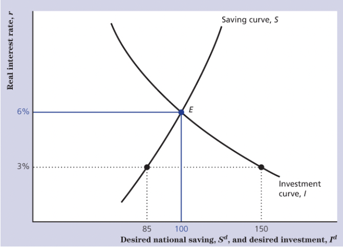
This point is shown as the intersection between the saving curve (Sᵈ) and investment curve (Iᵈ) — labeled as point E on the graph.
2. What Happens When G Increases
Government spending (G) is part of total output:
Y = C + I + G
If G increases, the government uses more of the economy’s resources, leaving less available for saving and investment.
From the saving formula:
Sᵈ = Y – Cᵈ – G
If G rises (and Y doesn’t change), desired saving (Sᵈ) decreases — meaning the government is saving less or borrowing more.
3. Effect on the Saving Curve
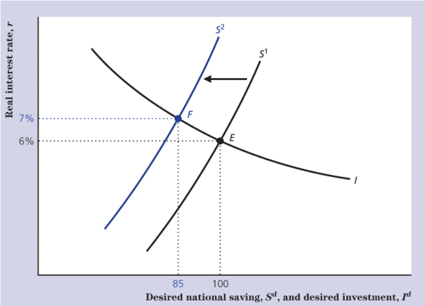
Because desired national saving falls, the saving curve shifts to the left — from S₁ to S₂ in the diagram.
This shift reflects that, at every interest rate, the economy saves less than before.
4. New Equilibrium
When the saving curve shifts left:
The new equilibrium point moves from E to F
The real interest rate (r) rises (from 6% to 7% in the diagram)
The equilibrium level of investment falls (from 100 to 85)
5. The Crowding-Out Effect
This outcome is called crowding out:
Higher government spending reduces the funds available for private investment.
As a result, both investment (Iᵈ) and sometimes consumption (Cᵈ) fall.
This is a saving–investment diagram, where:
The S curve (upward sloping) shows desired saving (Sᵈ) — households save more when the real interest rate (r) rises.
The I curve (downward sloping) shows desired investment (Iᵈ) — firms invest less when r rises because borrowing is more expensive.
The point where they meet (E) is goods market equilibrium (Sᵈ = Iᵈ).
2. What happens when new technology is invented
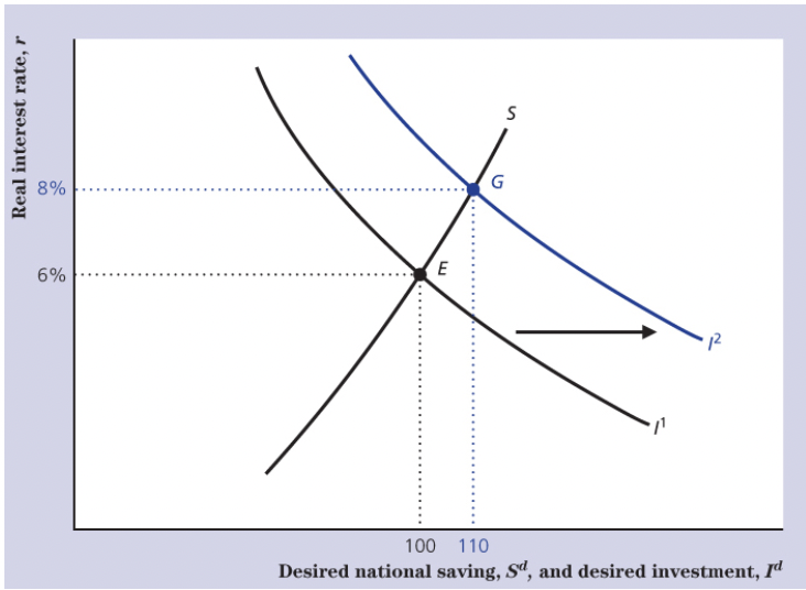
A technological improvement makes production more efficient and increases the expected marginal product of capital (MPKᶠ) — meaning capital becomes more profitable.
Because of this, firms want to invest more at every interest rate.
That means the investment curve shifts to the right, from I₁ → I₂ in the diagram.
3. The new equilibrium
The equilibrium moves from E to G.
The real interest rate (r) rises (from 6% to 8%).
The equilibrium level of investment also increases (from 100 to 110).
This shows that better technology encourages more investment — firms are willing to borrow and spend more on new equipment, machines, etc.
4. When would the investment curve shift left instead?
The investment curve (Iᵈ) shifts left when firms want to invest less at every interest rate.
This could happen if:
The marginal product of capital falls (technology worsens or becomes less productive).
There is an increase in corporate taxes.
Firms face higher uncertainty or lower business confidence.
The user cost of capital rises (for example, due to higher interest rates or depreciation costs).