Chapter 6

Owners of firms have multiple decisions to make:

• Firm structure

• Production methods

• Expansion strategies 🡪 (short-run adjustments + long-term investments)

• The volume of output to produce.

Economic theory helps firms make decision on production process, types of inputs to use and the volume output to produce.

6.1. Ownership and management of the firm

Firms 🡪 Organizations that turn inputs like labor + materials) into goods or services.

Types of firms

• Private: owned by people or other nongovernmental entities, whose goal is to make profit

• Public: Owned by governments or gov agencies

• Non-profit: Organizations that aren’t owned by the government but their goal isn’t to make profit but to pursue social or public objectives. Ex: Greenpeace,

Ownership for profit firms

For-profit firms in the private sector have three main legal structures:

1. Sole Proprietorship: Owned by a single individual. Ex: Small local shops.

2. Partnership: Jointly owned and controlled by two or more people. Ex: Law firms.

3. Corporation: Owned by shareholders who own shares (stock). Shareholders elect a board of directors, who hire managers. Owners have limited liability, protecting personal assets. Ex : Large companies like Apple or Microsoft.

Key feature of corporations is limited liability, (protecting owners' personal assets from the firm's debts) . This concept of limited liability serves as a strong motivator for people to invest in corporations because it minimizes their financial risk. Investors are more willing to buy shares, knowing that their potential losses are confined to the value of their investment.

Limited liability :the personal assets of the owners that can’t be used to pay for a corporation’s debt even if it goes into bankruptcy .

🡪 If a corporation faces financial difficulties or declares bankruptcy, the most shareholders can lose is the amount they invested in buying the company's stock. Their personal assets are shielded from being taken to pay the company's debts.

Management of firms

In small firms, owners often handle management, while larger corporations and partnerships typically have managers or management teams. Decision-making involves owners, managers, and supervisors, each with potentially conflicting objectives.

Ex: a manager may seek benefits that an owner might view as impacting profits negatively.

In corporations, the board of directors oversees managerial decisions, ensuring alignment with the firm's objectives. Shareholders hold the power to replace ineffective managers or influence policies through votes at annual meetings.

What owners want ?

Owners typically aim to maximize profit, represented as the difference between revenue (what the firm earns) and costs (what it pays for inputs). Profit maximization is crucial for staying competitive. Efficient production, achieving technological efficiency, is necessary for profit maximization. It means producing the current output level with the least amount of inputs based on existing knowledge.

While efficient production is necessary, it alone doesn't ensure profit maximization. Managers, often guided by economic decisions, determine how to produce at the lowest cost or with the highest profit(. This involves strategic choices in technology and input combinations.

6.2. Production

Firms use technology or production process to transform inputs (factors of productions) into outputs.

Here are the different types of inputs:

1. Capital services (K): Long-lived inputs like land, buildings, and equipment.

2. Labor services (L): Hours of work from managers, skilled, and less-skilled workers.

3. Materials (M): Natural resources, raw goods, and processed products consumed or incorporated in the final product.

Production function

Firms have many ways of transforming inputs into output. The production function shows the relationship between the number of inputs used and the maximum output that can be achieved

q=f(L,K)

🡪 The production function showcases the maximum output possible with given levels of labor and capital, focusing on efficient production processes. A profit-maximizing firm avoids inefficient processes and aims to use resources optimally.

Ex: Consider a smartphone manufacturing company with multiple production methods. In smaller setups, skilled workers assemble phones manually, while larger firms may introduce automated assembly lines. In advanced facilities, robots and advanced machinery, maintained by skilled technicians, handle intricate assembly processes.

The production function for such a firm, involving labor (L) and capital (K), might be expressed as q=f(L,K)),

q= nbr of smartphones produced

L= labor services 🡪 skilled + unskilled workers

K= capital 🡪 machinery + technology

Varying inputs over time

It’s easier for a firm to adjust its inputs in the long run than in the short run, because in the short run, a firm faces limits in adjusting its inputs, with at least one factor being practically unchangeable. This fixed factor is a fixed input, while those that can be easily adjusted are variable inputs. Conversely, the long run allows a firm to vary all factors of production.

Ex :.Imagine a bakery with a fixed-size oven (fixed input) and variable inputs like flour, sugar, and labor. In the short run, if the bakery wants to increase production, it can buy more flour and sugar or hire additional workers, but it can't immediately change the oven size. In the long run, the bakery can expand or replace the oven along with adjusting other inputs to meet changing demands.

In different industries, the time it takes to change inputs varies :

In industries like janitorial services that mainly rely on labor, they can easily adjust their workforce in the long term. For instance, if a cleaning company needs more employees due to increased demand, they can hire more workers relatively quickly.

However, in industries such as automobile manufacturing that heavily depend on complex machinery and factories, making changes takes a long time. For example, building a new car manufacturing plant or developing specialized equipment requires substantial time and investment, often spanning years.

In simpler terms, industries where the main input is people can adjust their workforce faster in the long run, while those relying heavily on machinery or infrastructure take much longer to make changes.

• Short Run: A short time frame where at least one factor of production cannot be practically changed by the firm.

• Fixed Input: A production factor that a firm cannot easily change or adjust during the short run.

• Variable Input: A production factor that the firm can readily adjust or change within the relevant short-run period.

• Long Run: An extended period in which a firm has enough time to adjust or change all factors of production as needed.

6.3. Short run production

In the short run, a company has fixed inputs, like capital or factory space, that can’t be altered immediately due to contractual obligations, technological constraints, or time needed for changes.

Companies may use the short run to make immediate production adjustments by varying only the variable inputs like labor, raw materials, or energy consumption.

Ex : hiring or firing workers, using overtime, or adjusting the quantity of raw materials without changing the overall capacity of the factory.

.

Scenario: a firm assembling computers with fixed capital (eight fully equipped workbenches) and variable labor. The short-run production function is given by q=f(L,K) where q is the output, LL is the amount of labor, and K is the fixed capital.

🡪 as shown in Table 6.1, with zero workers, no computers are assembled. Adding workers initially increases output, reaching a maximum of 110 computers per day with 10 or 11 workers. However, employing more than 11 workers becomes inefficient, decreasing production.

Marginal Product of Labor

a concept used to understand how an additional worker affects total output. Represents the extra output produced from adding/ hiring one more unit of labor (worker)

“If we add 1 more worker, how much are we producing “

MPL=∆q/∆L

EX: in Table 6.1, when the number of workers increases from 1 to 2 (∆L=1∆L=1), the output rises by ∆q=18−5=13. Therefore, the marginal product of labor is MPL=13/1=13.

In the short run, where capital is fixed, the focus is on how changes in labor impact output. Understanding MPL helps managers make decisions about hiring additional workers based on their contribution to overall production

Average product of labor

The average product of labor (APL) is another crucial measure for firms, representing the ratio of output (q) to the number of workers (L) used in production.

Represents the average output produced per unit of labor input.

🡪 provides iinfo on the productivity of labor, shows how much output, on average, each unit of labor contributes to the production process.

APL=

EX: The output (q) is given by 2L+1002L+100.

To determine APL:

1. Calculate APL: APL=qL=2(L+ΔL)+100L+ΔLAPL=Lq​=L+ΔL2(L+ΔL)+100​ Simplifying this expression yields APL=2APL=2.

2. Determine Marginal Product of Labor (MPL): To find MPL, considering an increase in workers by ΔLΔL, the change in output is Δq=2ΔLΔq=2ΔL. Thus, MPL=ΔqΔL=2MPL=ΔLΔq​=

Graphing the product curves

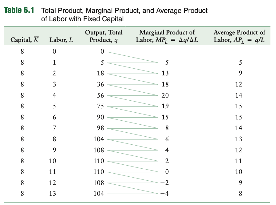In Figure 6.1, the production relationships with variable labor are illustrated. The total product curve (panel a) shows the amount of output that can be produced by a given amount of labor, reaching its peak at 110 computers with 11 workers. The dashed line indicates inefficient production with more than 11 workers.

Panel b of Figure 6.1 demonstrates the variation of the average product of labor (APL) and marginal product of labor (MPL) with the number of workers. The APL initially rises, indicating that output increases more than in proportion to labor due to factors like specialization. However, beyond a certain point, the APL falls as output increases less than proportionally to labor.

Geometric Relationship of Curves:

• Average Product and Marginal Product:

The point where the Average Product of Labor (APL) curve meets the Marginal Product of Labor (MPL) curve marks the peak of APL. At this spot, each worker achieves the highest average output, and MPL equals APL. After this point, APL decreases because each new worker contributes less to the average output than the current average.

• If AP=MP then AP at max. : When MPL equals APL, adding more workers doesn't change average productivity.

• If MP>AP then AP increasing : When MPL is higher than APL, adding more workers increases average productivity

• If MP < AP then AP decreasing : When MPL is less than APL, adding more workers decreases average productivity.

• Average Product and Total Product:

• The slope of the line from the origin to any point on the Total Product of Labor (TPL) curve for a specific quantity of workers represents the Average Product of Labor (APL) for that particular number of workers.

• EX ; if you draw a line from the origin to a point on the TPL curve that corresponds to a certain number of workers, the slope of this line gives you the APL for that specific quantity of workers.

• Marginal Product and Total Product:.

The slope of the tangent line to the Total Product of Labor (TPL) curve at a specific point represents the Marginal Product of Labor (MPL) at that particular level of output

• If you draw a tangent line to the TPL curve at a specific quantity of workers, the slope of this tangent line gives you the MPL at that level of labor input.

• when MP > 0 then TP is increasing. : When Marginal Product (MP) is positive (+), it means that adding more workers leads to an increase in Total Product (TP). Each additional worker contributes positively to the total output.

• When MP < 0 then TP is decreasing. : When MP becomes negative (-), it implies that further additions of workers result in a decrease in Total Product. This happens when additional workers cause inefficiencies or hinder the production process.

• When MP is at max then TP is at inflection point : At the maximum point of MP, Total Product (TP) reaches an inflection point, indicating the highest rate of change in TP. This inflection point represents the peak of productivity concerning the number of workers hired.

• When MP = 0 then TP is at a max : When MP reaches zero (0), Total Product (TP) is at its maximum. This occurs because MP turning from positive to zero signifies that adding more workers no longer increases output, indicating the peak of production efficiency.

Law of diminishing marginal return

The Law of Diminishing Marginal Returns states that as a firm increases a particular input while holding other inputs and technology constant, the corresponding increases in output will become smaller eventually. So, if only one input is increased, the marginal product of that input will diminish over time.

EX: In Table 6.1, as the firm goes from 1 to 2 workers, the marginal product of labor increases (from 13 to 18), but beyond a certain point (4 workers), it starts to fall. The law of diminishing marginal returns suggests that each additional worker contributes less and less to the total output.

Diminishing Marginal Returns vs. Diminishing Returns:

Diminishing marginal returns is when you add more of something (like labor or resources) while keeping other factors constant, each extra bit you add doesn't boost production as much as the previous ones did. However, this doesn't automatically mean that the total amount produced will decrease. It might still increase, but at a decreasing rate.( while there might still be an increase, it's happening at a slower pace compared to before.)

It's a concern because adding more of a particular input might not increase production by as much as before. But in real life, advancements in technology and using different inputs together that can help lessen this effect.

EX: in farming, using better techniques or combining different resources can help maintain or increase overall production despite facing diminishing returns from each additional unit of input.

6.4. Long run production

In the long run, both labor and capital are variable inputs, allowing a firm to produce a given level of output through different combinations of these inputs. This flexibility allows for substitution between inputs, similar to how consumers can substitute between goods to maintain a certain level of utility.

Isoquants

DEF: represents the different combinations of labor and capital that allow a firm to produce a specific level of output.

🡪shows combinations of K+L and the technological tradeoff between the 2

(How much capital would be required to replace a unit of labor a a certain production point to generate the same output ?).

Isoquants share several properties with indifference curves, which are used in consumer theory.

Isoquant vs indifference curves 🡪 The difference is that isoquants maintain a constant level of output, while indifference curves maintain a constant level of satisfaction or utility.

Properties of isoquants:

• Output Level: Isoquants farther from the origin mean higher levels of output. This is because the firm utilizes more inputs efficiently to achieve increased production.

• Non-crossing: Isoquants do not intersect or cross. This property ensures efficiency because if two isoquants were to intersect, it would imply that the same level of output could be produced with the same combination of labor and capital, violating the principle of efficiency.

• Downward Sloping: Isoquants slope downward. This characteristic is essential because it reflects the trade-off between labor and capital. As more of one input is used, less of the other is required to maintain the same output level.

• Shape and Substitutability: The curvature of isoquants demonstrates the firm's ability to substitute one input for another.

• Perfect substitutes : result in straight-line isoquants,

• fixed-proportions production functions (no substitutes) : lead to right-angle isoquants.

• Most isoquants are convex, sloping downward and curving away from the origin, indicating imperfect substitution between inputs.

In all, isoquants provide a visual representation of a firm's production capabilities and the various combinations of labor and capital that lead to constant output levels.

Marginal rate of technical substitution (MRTS = slope of isoquant) : Measures how easily a firm can exchange ne input for another while keeping output constant

MRTS=

Illustration: In Figure 6.4, the isoquant for a service firm producing 10 units of output is examined. The points a, b, c, d, and e represent different combinations of labor (L) and capital (K). The slope of the isoquant at each point corresponds to the MRTS.

Substitution Example: Moving from point a to b, the firm can produce the same output using six fewer units of capital (∆K = -6) if it hires one more worker (∆L = 1). Therefore, the MRTS at this point is -6.

As the firm increases labor along the isoquant (EX: moving from b to c or c to d), the MRTS declines.

🡪Diminishing MRTS : implies that each additional worker contributes less to the reduction in the use of capital, highlighting the challenge of replacing remaining capital with labor.

Special Case: Isoquants with perfect substitutes do not exhibit diminishing MRTS since the inputs remain perfect substitutes, and neither becomes more valuable in the production process.

6.5. Returns to scale

Returns to scale refers to how changes in inputs like labor and capital affect the output in a production process that employs the same technology. It's a way to measure how efficiently a firm can convert inputs into outputs.

Increasing Returns to Scale:

• If a firm doubles its inputs (EX:labor, capital) and output more than doubles.

• This implies that as the firm expands its scale, it becomes more efficient, possibly benefiting from factors like specialization and resource pooling.

f(2L,2K)= 2f(L,K) = 2q

• Ex: a software development company that enhances its workforce by 20% and, as a result, experiences a 30% increase in developed software products. This scenario reflects increasing returns to scale, possibly due to improved collaboration among team members or specialized skills that enhance productivity as the team grows.

Constant Returns to Scale:

• If a firm doubles its inputs and output exactly doubles, it indicates constant returns to scale.

• This suggests that the firm maintains the same level of efficiency as it scales up, achieving a proportional increase in output.

• Ex : Imagine a pizza shop that doubles both its oven capacity and the number of chefs while keeping all other factors constant. If this doubling of inputs results in exactly double the number of pizzas produced without any change in efficiency, it demonstrates constant returns to scale.

Decreasing Returns to Scale:

• occur when doubling inputs results in less than a doubling of output.

• This implies that as the firm expands, efficiency may decline due to issues like coordination challenges or diminishing returns to inputs.

• Ex : a factory that manufactures furniture. If the factory doubles its production capacity by expanding its machinery and labor force but sees only a 50% increase in the furniture output, it signifies decreasing returns to scale.

Varying returns to scale

The variation in returns to scale showcases the complexity of production dynamics as firms change in size. Small firms benefit from growth and specialization, but as they expand, challenges related to management and coordination might arise, leading to diminishing returns.

6.6. Productivity + technical change

Differences in technology and managerial practices contribute to variations in firms' output from the same inputs. Technological advancements and managerial innovations enable firms to increase productivity, producing more with the same resources. This phenomenon is known as technical change or technological progress. Firms embracing these changes often outperform others by optimizing their production processes.

Relative productivity

Efficiency is crucial for maximizing profit, but firms within a market might still differ in productivity. Factors like management strategies, access to innovations, and external influences can impact relative productivity. Market competition plays a significant role – in competitive markets, less productive firms exit, leaving equally productive ones. In less competitive markets, firms with varying productivity levels may coexist. Factors such as work rules, discrimination, regulations, or institutional restrictions can influence relative productivity among firms.

Innovations

the pursuit of efficiency, firms strive to incorporate the latest technological and managerial advancements in their production processes. Technical progress, arising from innovations, enables firms to produce more output with the same inputs. Whether through new inventions, technical innovations like robotics, or improved management practices, technical progress plays a vital role.

Ex: a firm may produce 10% more output this year with the same inputs due to a new invention.

There are different types of technological progress :

• Neutral Technical Change:a technological improvement or advancement that increases productivity without favoring any particular type of input over others. It equally affects all factors of production, like labor and capital, leading to an overall increase in efficiency without changing the ratio of inputs used in production.

• Non-neutral Technical Change: When innovation affects the productivity of one input but not the other

Ex: if a company has a new machine that boost the productivity of capital but reducs labor because of the implementation of the machine they need less workers (labor saving technical change)

There are 2 steps that a firm takes in order to choose how to produce outputs efficiently:

1. Identifying TECHNOLOGICALLY EFFICIENT Production Processes: The firm aims to find the most effective and efficient ways to produce a specific output level.

2. selecting the most ECONOMICALLY EFFICIENT production process among the technologically efficient options: jAfter finding effective ways to produce what they want, the firm picks the most cost-efficient method. They use info from how inputs create output (production function) and input costs to choose the way that minimizes expenses while keeping output at the desired level. It's about finding the cheapest way to make things without compromising on the quantity they want to produce.

economically efficient :minimizing the cost of producing a specified amount of output

Chapter 7

7.1. The nature of costs

Cost analysis in economics involves measuring a company's expenses related to production. Economists and business professionals differ in how they evaluate costs. Economists consider all relevant costs, while managers often focus on financial statements tied to tax laws and shareholder interests.

To create products, a company spends on inputs like labor, capital, energy, and materials. The cost of each input is found by multiplying its price by the quantity used. For instance, if labor costs $20 per hour and the firm uses workers for 100 hours, the labor cost would be $20 * 100 = $2,000 per day. These are explicit costs, representing direct payments for inputs.

Explicit costs : These are the straightforward, tangible costs, like the money spent on purchasing machinery. Ex: rent , material, wages

Implicit costs : are not actual cash payments but represent the value of opportunities a business misses when it uses its resources in a certain way. They are about what the company gives up by choosing one option over another. (They're the opportunity costs—the benefits or profits a company forgoes by choosing one alternative over another.)

Ex if a business owner decides to use their own building for their company instead of renting it out to another business, the implicit cost is the potential rental income they've given up.

Opportunity cost

Opportunity cost : the value of the best alternative use of a resource. It encapsulates both explicit costs (direct, out-of-pocket payments for inputs) and implicit costs (opportunity value of forgone alternatives).(I t's the cost of choosing one option over another)

Ex; If you decide to buy a pizza instead of a burger, the opportunity cost is the taste of the burger that you gave up by choosing the pizza.

EX: imagine Maoyong, who owns a firm, pays himself a salary of $1,000 monthly but could earn $11,000 elsewhere. The opportunity cost of his time isn't the $1,000 he pays himself but rather the $11,000 he could earn elsewhere, highlighting the concept of opportunity cost.

Finding opportunity cost means figuring out what you miss out on by choosing one thing over another. It's about understanding the benefits you give up from the options you didn't choose.

Scenario-🡪 Meredith's firm sends her to a conference, including a free class on pricing derivative securities. However, she could attend a talk by Warren Buffett at the same time. Meredith values Buffett's talk at $100 but the ticket costs $40. If she chooses the derivatives class, her opportunity cost is $60 ($100 - $40), representing the benefit she gives up by not attending Buffett's talk.

Opportunity cost of capital

Opportunity cost of capital refers to the value of the best alternative use of durable assets like equipment or land, typically used over a long period. Determining this cost involves considering allocation of purchase cost and accounting for changes in asset value over time.

Ex: When a company chooses to rent capital assets (such as machinery, vehicles like trucks, or equipment), the monthly rental payment it makes essentially represents the cost the company incurs to use that particular asset for a month. This rental payment reflects the opportunity cost, as it signifies the value of using that asset for that period.

Renting capital assets simplifies the financial aspect for the company. Instead of dealing with the complexities of allocating or spreading out the purchase cost of an asset over its entire useful life, which is the case when buying it outright, the rental cost is a clear and immediate expense. This simplicity in accounting helps in managing and understanding the ongoing monthly expenses more easily.

Sunk Cost: It's money spent in the past that cannot be recovered. Sunk costs have already occurred.

Ex : Buying a gym membership for a year and then deciding not to go anymore. The money spent on the membership is a sunk cost because it's already paid and cannot be recovered, regardless of using the gym or not.

7.2. short-run costs

In the short run, a firm faces costs that increase as it produces more. It's more expensive to increase output in the short run because certain inputs, like capital, cannot be adjusted. This contrasts with the long run, where all inputs are flexible.

Short run cost measures

To produce a given level of output a firm incurs costs for fixed and variable inputs (in the

Shortrun :

• a firm faces fixed costs that stay the same regardless of output and variable costs that change with the quantity of output produced.

Ex: expenses for resources that can't be adjusted in the short run, like land or equipment.

VC= w x L

• Variable costs:fluctuate with the level of output, involving items such as labor and materials.

• The total cost (TC) to produce a specific quantity of output is the sum of fixed cost (F) and variable cost (VC).

• EX: if a firm has a fixed cost of $48 and a variable cost that rises from $25 for one unit to $46 for two units, the total cost for producing two units would be $94 ($48 + $46).

TC= F+VC

To decide how much to produce, a firm uses several measures of how its costs varies with the level of output.:

or w x L/Q

• Marginal cost (MC): is the change in total cost when producing one more unit of output. It helps firms decide if it's profitable to adjust their output.

FC/Q or w x L/Q

• Average fixed cost (AFC) : is the fixed cost divided by the number of units produced, decreasing as output increases.

VC/Q

• Average variable cost (AVC): is the variable cost divided by the quantity of output produced, fluctuating with output changes.

• Average cost (AC) or average total cost : is the sum of AFC and AVC, showing the overall cost per unit of output. These cost measures assist firms in determining their profitability concerning the price they receive for their products.

TC/Q

Short run cost curves

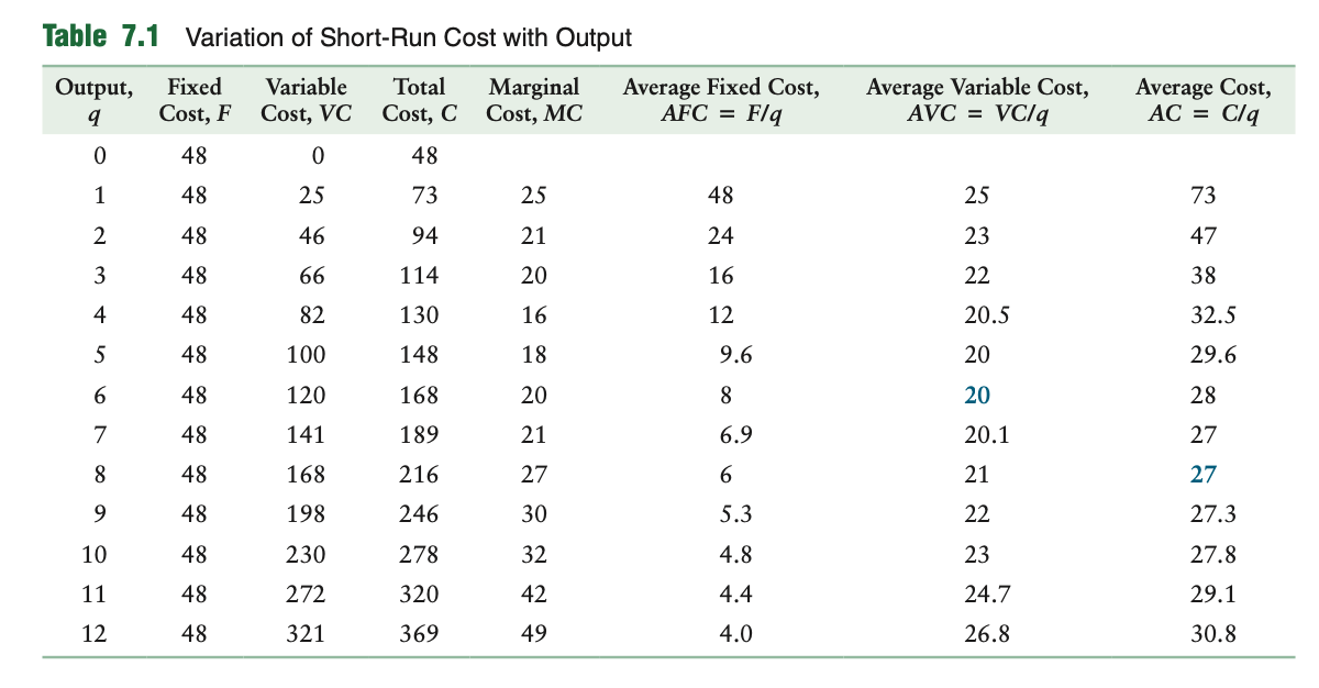
The short-run cost curves show different types of costs a firm faces at various output levels. In Figure 7.1, Panel a shows fixed cost as a horizontal line at a constant value ($48), while the variable cost curve starts from zero and rises with output. The total cost curve, representing the sum of fixed and variable costs, runs parallel to the variable cost curve.

Panle A

• Fixed Cost Curve 🡪 A straight line representing costs that do not change with changes in output. It remains constant regardless of the production level.

• Variable Cost Curve 🡪 Starts at zero when production is at zero and increases with output because these costs vary with the number of units produced.

• Total Cost Curve 🡪 is a parallel line to the VC-curve, which is “amount of the FC” higher than the VC.

Panel B

• Average Fixed Cost curve 🡪 Decreases/falls as output rises because the fixed costs are spread over more units as production increases.

• Average Cost curve 🡪 Sum of the Average Fixed Cost curve and the Average Variable Cost Curve

• Falls when MC < AC and rises when MC > AC

• Marginal Cost Curve 🡪 the slope of tangent TC is equal to the slope of the tangent VC

• Average Variable Cost curve 🡪 slope of line through origin and VC

  • It falls when the MC < AVC and it rises when MC > AVC

  • MC intersects AVC at its min

The Relationship Between Marginal Cost and Average Cost:

• When MC is below ATC or AVC, the average cost decreases.

• When MC is above ATC or AVC, the average cost increases.

• At the minimum point of the average cost curve, MC equals ATC.

The production function defines a firm's cost curves. It shows the relationship between inputs required to produce a specific output level.

In the short run, a company deals with costs that can be changed based on production levels. These costs are termed as variable costs. A key variable cost for many companies is labor expense, which changes based on the number of hours worked by employees and their wage rate.

Variable Cost (VC) = Wage per hour (w) * Number of hours of labor (L)

Ex: if a firm pays its workers $15 per hour and employs 100 hours of labor, the variable cost would be $15 * 100 = $1,500.

• Variable Cost Curve: It shows how costs go up when a company hires more workers. As more workers are hired, the cost for each additional worker might not produce as much extra output, leading to higher costs per unit.

• Marginal Cost (MC) Curve: This displays how the cost changes when making one more product. At first, adding more workers might reduce costs because they're more productive. But beyond a point, adding more workers leads to less extra output for each new worker, causing costs to rise.

• Average Variable Cost (AVC) Curve: It shows the cost per item produced. When each worker produces more, the cost per item decreases, and when each worker produces less, the cost per item increases.

• Average Total Cost (AC) Curve: This combines fixed and variable costs. It forms a U-shape because at low levels of production, fixed costs spread over fewer items, and at high levels, diminishing returns cause variable costs to rise per item

The relationship between these curves is such that:

When the Marginal Cost is below the Average Cost, the Average Cost tends to decrease.

When the Marginal Cost is above the Average Cost, the Average Cost tends to increase.

If Marginal Cost equals Average Cost, the Average Cost curve is at its minimum point.

Taxes

• Impact of Tax on Costs:

  • If a tax is imposed per unit of output (e.g., $10 per unit), it increases both average variable cost (AVC) and average cost (AC) by that tax amount ($10).

  • Marginal cost (MC) and average cost curves shift upward by the tax amount. However, the points where these curves reach their lowest (minimum) values don't change despite the tax increase.

• Franchise Taxes' Effect:

  • Franchise taxes, which are fixed lump-sum payments unrelated to output, only impact fixed costs.

  • These fixed taxes don't influence how costs change with each extra unit produced (marginal cost curve) but affect the fixed cost part of the average cost curve.

  • As a result, after-tax average cost curve reaches its minimum at a higher production level compared to the before-tax curve due to the additional fixed tax payment.

7.3 Long-Run Costs

All Costs are Avoidable in the Long-Run

🡪fixed costs in the long-run are avoidable (rather than sunk, as in the short run)

1. Fixed Costs in the Short Run:

   • In the short run, fixed costs are often considered sunk costs.

   • Example: Rent payments for a restaurant space, which remain unchanged regardless of whether the restaurant operates or not. These costs are unavoidable in the short run.

2. Fixed Costs in the Long Run:

   • However, in the long run, fixed costs are avoidable.

   • Example: The same rent for the restaurant space can be avoided in the long run by shutting down the restaurant. Unlike the short run, where the rent is paid irrespective of operations, in the long run, the firm has the flexibility to avoid such fixed costs by ceasing operations.

The difference between the short run and the long run regarding fixed costs is that in the long run, a firm has more flexibility and can adjust its costs, including avoiding certain fixed costs by making different decisions such as shutting down operations.

1. Long Run Total Cost Equals Long-Run Variable Cost:

   • In the long run, the total cost of production is equivalent to the long-run variable cost.

   • This denotes that all costs incurred in the long run, when the firm can adjust all inputs including capital, are considered variable costs. There are no fixed costs in the long run.

2. Lower Long-Run Cost When Using "Wrong" Capital in Short Run:

• Sometimes, when a business can't adjust certain things (like equipment or machinery) in the short term, it might end up spending more money than necessary.

• But when it has the chance to adjust everything in the long term, it might spend less because it can make better choices about how it uses its resources.

Minimising Costs

• A firm can produce a given level of output using many different technologically efficient

combinations of inputs, as summarized by an isoquant

• From the technologically efficient combinations of inputs, a firm wants to choose the bundle withthe lowest cost of production →the economically efficient combination of inputs.

• A company can make the same amount of stuff using various combinations of tools, workers, and resources.

• Out of all these combinations that work efficiently, the company aims to pick the one that costs the least to produce - that's the most economical way to make their product. This chosen combination is called the economically efficient mix of inputs.

Isocost Line

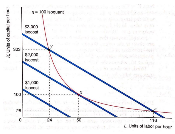
All the combinations of inputs that require the same (iso) total expenditure (cost)

The cost of producing a given level of output depends onthe price of labour and capital

C = wL + rK.

3 properties:

1. Where the isocost line hits the axes depends on the firm’s cost

2. and on the input prices.

3. Isocosts farther from the origin have higher costs.

4. Slope of each isocost is the same; if a firm increases labour,decreases in capital

∆K = -w/r ∆L or ∆K/∆L = -w/r

→slope depends on input prices

both isocosts and budget lines are straight lines whose slopes depend on relative prices

difference: consumer has a single budget line determined by income, while a firm faces many

isocost lines each of which corresponds to a different level of expenditures it might make.

Combining Cost and Production Information

The firm can use any of three equivalent approaches to minimise its cost:

Lowest-Isocost Rule:

• Pick the bundle of inputs where the lowest isocost line touches the isoquant

• firm minimises its cost by using the combination of inputs on the isoquant that is on the lowest isocost line that touches the isoquant

• If an isocost line touches the isoquant twice, there must be another lower isocost line that also touches the isoquant

Tangency Rule

• Pick the bundle of inputs where the isoquant is tangent to the isocost line

• Firm chooses the input bundle where the relevant isoquant is tangent to an isocost line to produce a given level of output at the lowest cost

• To minimise its cost of producing a given level of output, a firm chooses its input so that the

• MRTS equals the negative of the relative input prices: MRTS = - w/r.

Last-Dollar Rule

• Pick the bundle of inputs where the last dollar spent on one input gives as much extra

• output as the last dollar spent on any other product. The tangency rule can be interpreted

• in another way: MRTS = - w/r = - MPL/MPK  MPL/w = MPK/r.

• If the isoquant is not smooth, the lowest-cost method cannot be determined by using the tangency rule or the last-dollar rule

• The lowest-isocost rule always works, even when isoquants are not smooth

Factor Price Changes

The change in a price does not affect technological efficiency, so it does not affect the isoquant, only the isocost line is different

The Long-Run Expansion Path and the Long-Run Cost

Function

• Expansion path: line through the tangency points,the cost-minimising combinations of labour and capital for each output level.

• long-run cost function shows relation between the cost (isoquant) and the total output (isocost line).

The Shape of Long-Run Cost Curves

• shapes of the average cost and marginal cost curves depend on the shape of the long-run cost curve

• The long-run average cost curve falls when the long-run marginal cost curve is below it and rises when the long-run marginal cost curve is above it.

• the marginal cost crosses the average cost curve at the lowest point on the average cost curve

• Why does the average cost curve first fall and then,rise? →key reason is that the average fixed cost

7.4 Lower Costs in the Long Run

A firm’s long-run decisions determine its short-run cost. Short-run cost is at least as high as long run cost and is higher if the “wrong” level of capital is used in the short-run.

Long-Run Average Cost as the Envelope of Short-Run Average Cost Curves

• long-run average cost is always equal to or below the short-run average cost – if there are many possible SRAC, the LRAC will be smooth and U-shaped

• the LRAC includes one point from each possible short-run average cost curve. This point, however,is not necessarily the minimum point from a short-run curve

Short-Run and Long-Run Expansion Paths

long-run cost is lower than the short-run cost because a firm hasmore flexibility in the long run

short-run: firm can only change input of one variable, therefore, the expansion path of short-run output is horizontal – to double its output, it must increase its labour

relatively more and cost doubles relatively more

long-run: doubling inputs, doubles output, the long-run expansion

path is upward sloping

The Learning Curve

• Learning by Doing: the productive skills and knowledge that workers and managers gain from experience

• A firm’s average cost may fall over time due to learning by doing

• Learning is a function of cumulative output: the total number of units of output produced since the product was introduced

• relationship between average costs and cumulative output

• If a firm is operating in the economies of scales section of its average cost curve, expanding output

lowers its cost for two reasons