Chapter 20
Khalid keeps a spreadsheet to record his expenses and to plan for future spending. This spreadsheet is split into two separate sheets, which he has named Plan and Model. Plan contains details of his future spending. Model contains a model of his income and expenses
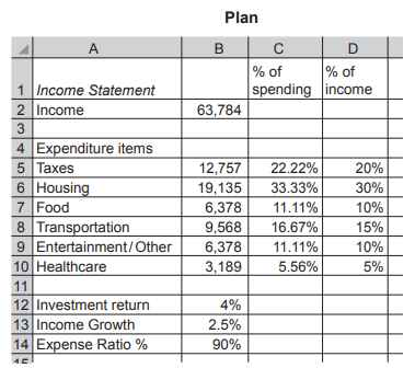
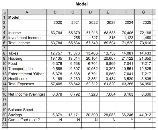
(a) Khalid has entered a formula in cell C4 of the Model sheet. The formula is B4+(B4*Plan!$B13) Explain, in detail, what the formula does. Include in your answer an explanation of why the $ and the ! are used in the formula.
It calculates the 2021 income in the Model sheet by increasing the 2020 income by 2.5%
The 2.5% is taken from the Income Growth cell in the Plan sheet
The $ is needed as the column B needs to be retained when the formula is replicated
The ! is needed to show that the data is being taken from a different worksheet
(b) He is saving up to buy a new car; this will cost at least $35,000. Khalid has entered a formula in cell B21 of the Model sheet. The formula is IF(B20>35000,"Y","N") Explain, in detail, what the formula does.
the formula automatically displays a Y
if the Savings cell/B20 is greater than $35 000
otherwise it displays an N
(c) Khalid is planning to create an appropriate graph/chart to be placed in a new sheet. The graph/chart will display the % of income and the names of the expenditure items from the Plan sheet. Identify the most appropriate graph/chart he could use and describe the steps he needs to take to produce this graph/chart in a new sheet.
Pie chart
steps he needs to take to produce this graph/chart in a new sheet.:
Select Plan sheet
Highlight A5:A10
Press CTRL and highlight D5:D10
Click on insert chart
Select pie chart
Choose style of chart
Add a title
Add data/axes labels
Add legend
Add a name for the new sheet
Right click on the chart and move to a new sheet or copy and paste in the new sheet
answer must have the last point to get all marks
The teacher has created a formula in the spreadsheet that calculates the cost of purchasing a number of different items. She has created a formula that:
subtracts the discount per item from the price of the item to find the cost of the item
then multiplies the cost of the item by the quantity.
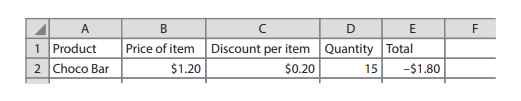 The formula she enters into cell E2 is:
=B2-C2*D2
When this formula is entered into cell E2 the result is not what she expected. The result should
be $15.00. Explain why the result was not $15.00
Brackets/parentheses missing around B2-C2
Multiplication was carried out first then the subtraction
The order of calculation should follow BODMAS/BIDMAS/PEMDAS
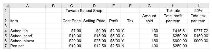
Tawara school has a shop that sells items needed by pupils in school. Part of a spreadsheet with details of the items is shown
 Write down the number of rows that are shown in the spreadsheet that contain text
6 rows
Write down the number of columns that are shown in the spreadsheet that contain text
8 columns
Tax is paid on certain items sold in the shop. The tax rate that has to be paid is 20% of the selling price. If tax is to be paid on an item, then ‘Y’ is placed underneath the Tax heading.
The formula in I4 is: IF(F4=''Y'',($I$1*D4*G4),'''')
Explain, in detail, what the formula does.
If Tax is payable then//If F4 is equal to "Y" then
If true the tax is paid
Multiply the rate of tax/I1 by the selling price/D4
… by the amount sold/G4
If Tax is not payable//If F4 <>"Y"//Else//Otherwise …
… then display a blank
… the tax is not paid
Explain the steps that need to be taken to display cell H4 as US dollars.
Highlight/select cell H4
Select format cells
Select currency/accounting
Select dollar/USD icon
Explain the differences between a VLOOKUP function and a LOOKUP function.
LOOKUP allows for horizontal and vertical searching whereas VLOOKUP allows for vertical searching
LOOKUP does not require an index value/only works on the second row/column whereas VLOOKUP requires an index value
LOOKUP usually only works when the data is sorted
VLOOKUP only returns data to the right of the searched column
VLOOKUP user can select either an approximate or exact match to the lookup value
A spreadsheet contains a list of staff and the rooms they work in at a school.
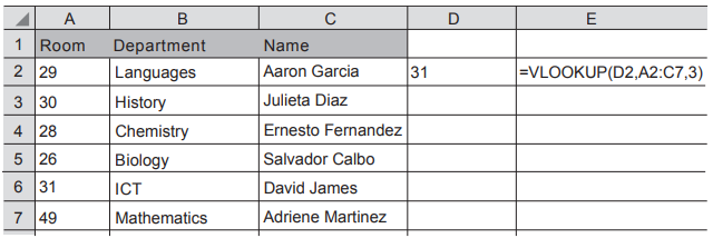 (i) Explain, in detail, what the formula in cell E2 does.
The formula looks up the value in D2 in the (range) A2 to A7
And returns the corresponding value
In the 3rd column/Column C
(ii) When certain room numbers are typed into cell D2 unexpected results appear in cell E2. Suggest improvements that could be made to ensure the correct result is displayed.
Add FALSE/0 to the end of the formula – 1 mark
Sort the range into ascending order of column A – 1 mark
A teacher in the school has created a spreadsheet to display whether a student has good timekeeping when arriving at lessons. He has produced a formula but thinks it could be improved. The formula is:
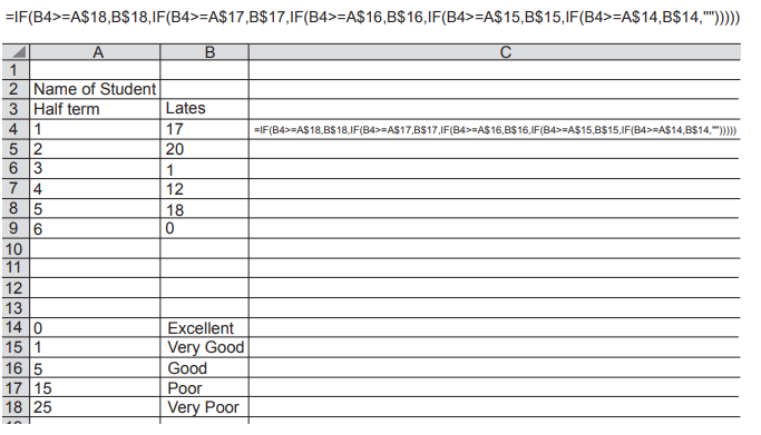 (c) Write down the value that should appear in cell C4
Poor
(d) The teacher has improved the formula and has typed in =VLOOKUP(B4,A$14:B$18,2) Explain the advantages of using this formula compared to the original one
Quicker to type in the formula
Fewer mistakes when typing in the formula
Easier to spot mistakes
Easier to expand the range
Takes up less storage space
Easier to remember when retyping
You are creating a presentation on the World Games. You have created a spreadsheet showing the number of gold, silver and bronze medals awarded to different countries. You are planning to create a graph in the presentation showing the country, the number of gold medals and the total number of medals.
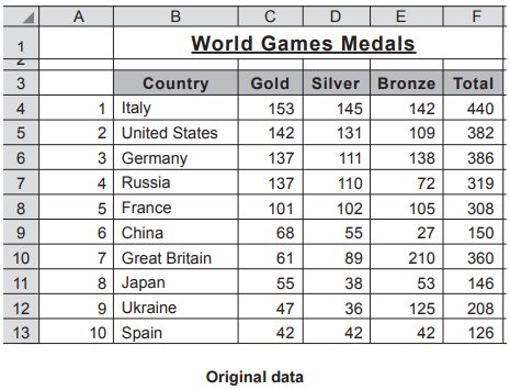 (a) Explain how you would create a vertical bar chart, showing the name of the country, the number of gold medals and the total number of medals awarded to each country, on a new slide in the presentation.
Max four from:
Open spreadsheet
Load the file
Select B3 to C13
Then hold CTRL and select F3 to F13
Click insert then click bar chart/graph
Select the format/type of chart/graph
Highlight the chart/graph
Copy the bar chart/graph
Max four from:
Open the presentation software
Add a new slide
Click on new slide
Paste the bar chart/graph
Add titles/legend/axes labels
Save the file
(b) The total number of medals has been calculated manually and entered as a value. This could lead to errors. Explain how you could create a formula to calculate the total number of medals awarded for Italy, using only the mouse
Click on the cell F4
Select formulas
Click Autosum/Σ
Check the correct range has been highlighted/highlight/drag C4 to E4
Click ✓
(c) Explain how the data could be sorted by the total number of medals won by each country. The country with the largest number of medals should be at the top of the list.
Highlight B3 to F13
Click Data then Sort
Select data has headers
Sort by Total/Column F
Select Largest to smallest/Descending/Z to A
Click OK/enter
A computer system is being created to calculate the scores in a diving competition. Every dive by an athlete is awarded a score out of 10 by each judge.
The system is being tested using live data. An athlete completes his dive with a difficulty of 3.4 and achieves the following scores, which are displayed in a spreadsheet
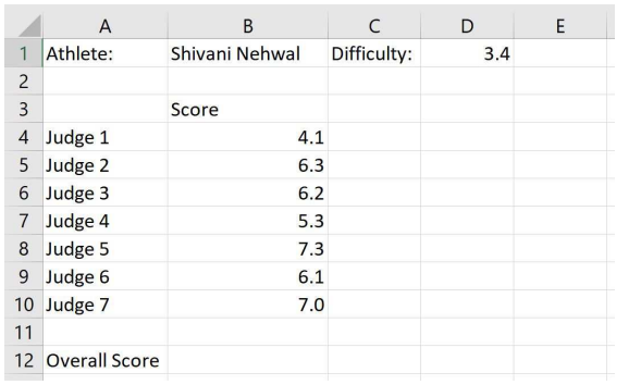 (a) Before the overall score is calculated the judges’ scores need to be sorted into ascending order. Describe the steps that would be carried out to sort the data into ascending order.
Highlight cells A4 to B10
Click on the down arrow//Click on Custom Sort
Select column B
Select smallest to largest/A ⬇ Z
(b) Cell B12 contains the formula, ROUND((SUM(B5:B9)*D1),1).
Explain what the formula in cell B12 does
Totals cells B5 to B9
Multiplies by cell D1
Rounds the value to 1 decimal place
(c) The judges’ score column will be tested using normal, abnormal and extreme data. Explain, giving examples of test data which would be used, what is meant by:
Abnormal test data
data that is outside the range//Unacceptable data//Data of the wrong type
example: greater than 10, negative numbers, letters, symbols
Extreme test data
data that is on the boundary of acceptability
example: 10
The student has transferred the data into a spreadsheet in order to create a graph.
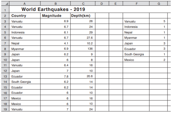 (a) She has entered a formula in cell G3. The formula is
COUNTIF(A$3:A$19,F3)
Explain in detail what the formula in G3 does. Include in your answer an explanation of the use of the $ sign.
The formula counts the number of times
Vanuatu/contents/value of F3
Appears in the country list/A3 to A19
The $ allows the range to remain static if replicated/search in the same range if replicated
(b) The student is creating an appropriate chart/graph of the data in cells F3 to G10.
Write down the steps she needs to take to produce a chart/graph of the data on the same sheet. Your answer must include examples of an appropriate title and labels.
Max four from:
Highlight F3 to G10
Click Insert Chart
Click Bar chart//column graph
Select layout/type of bar chart
Add title to the chart
Add axes
Add a legend
Save the chart
Three from, for example:
Title – Earthquakes in 2019
X/horizontal axis label – Countries
Y axis label/vertical – Number of earthquakes