Unit 5: Factor Markets
(5.1) Intro to Factor Markets
factor market graphs convey same info from units 1-4, just looks at products in a factor perspective
households own factors of production
h earn income by selling factors in resource market (EX: selling labor for wages)

marginal revenue product (MRP): extra revenue that firm gains when firm hires 1 additional worker/resource
formula: P * MR (change in revenue) = MRP
true whether product market is perfectly/imperfectly competitive
marginal factor or resource cost (MFC or MRC): additional cost paid by firm when it hires additional worker/resource
EX: wage for labor
MRC = TFC (price) / additional Q (usually +1)
MRP = MRC → MR = MC (profit maximizing quantity)
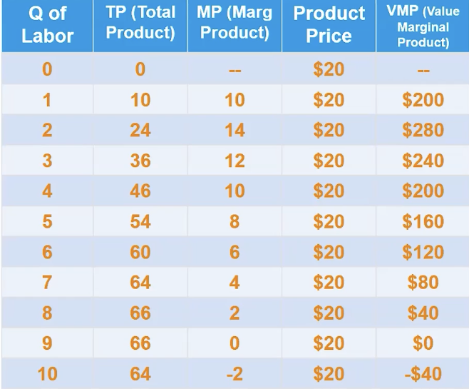
total product: amount produced with given amount of workers
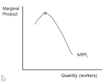
marginal product: change in total product that results in an additional worker/resource
table indicators:
increasing returns = increasing marginal product
diminishing returns = marginal product decreases (or diminishes)
negative returns = marginal product is a negative integer
in perfect competition:
P (price) = MR means perfectly competitive product market
MP * MR = MRP is the same as MP * P = VMP (value marginal product) in perfect competition
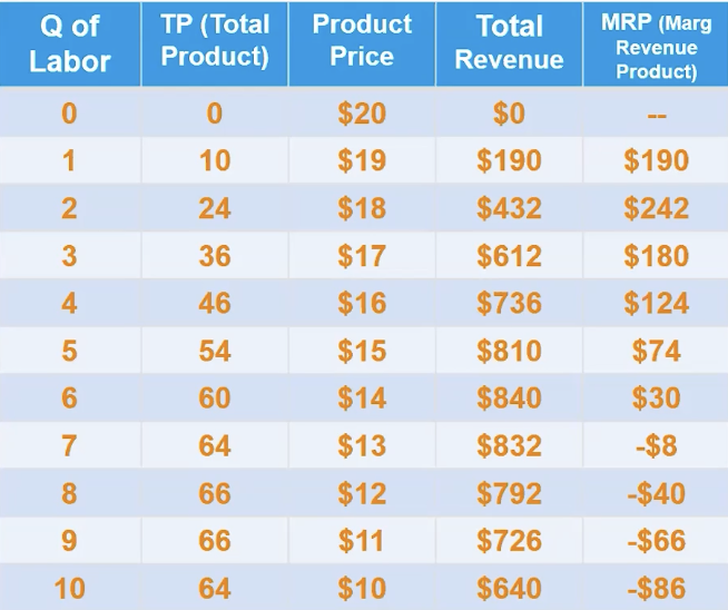
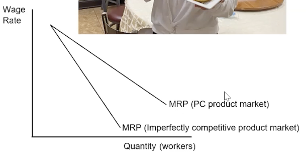
in imperfect competition:
downward sloping demand curve → firm needs to lower the price to sell additional units
TP (total product) is Q
P * Q = TR (total revenue)
change in TR with 1 additional worker is MRP
P > MR → MRP is focused on
MRP = (change in TR) divided by (change in quantity of labor)
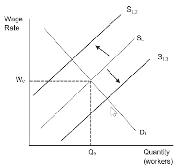
(5.2) Changes in Factor Demand/Supply
derived demand: demand of resource from product demand
effects: productivity (MPP) and output price (MRP)
MPP (marginal physical product) = change in total product / change in quantity (usually +1)
MRP (marginal revenue product) = MPP * MR
diminishing returns = output increases at a decreasing rate (MPP decreases) with additional input
demand determinants → MR
change in number of consumers
price of related good
increase if more expensive, decrease if not
government regulations
decreases productivity of workers → decreases demands
improvements in education
increase productivity of workers → increases demand
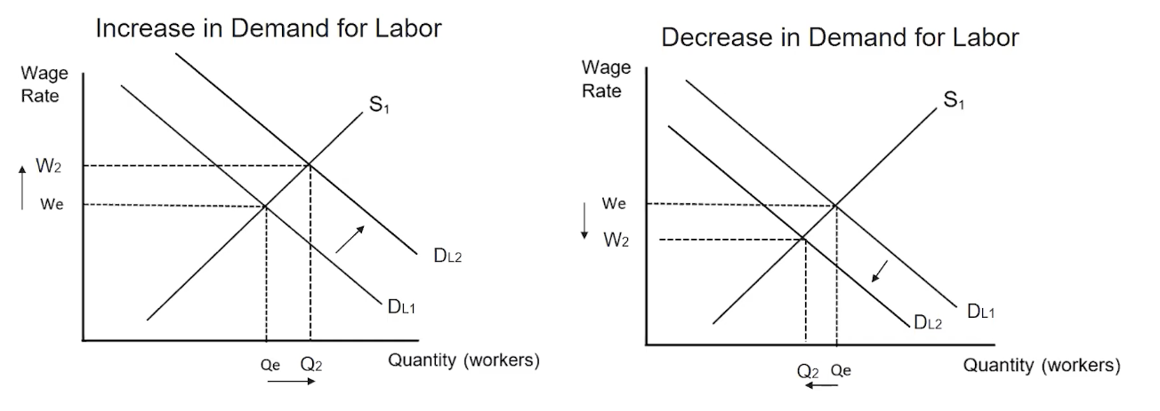
5 supply determinants
leisure (choosing not to work)
opportunity cost for work
increase in leisure → less in supply
number of alternative options
decrease in supply of one industry → increase in supply of another
age distribution
more retiring workers → less new workers entering
education
more years spent at universities → decrease in supply of labor
changes in skill levels
immigration
increase in immigration → increase in workers (vice versa)
(5.3) Profit-Maximizing Behavior in Perfectly Competitive Factor Markets
wage takers: workers that are selling labor at set price
perfectly competitive supply curve
TFC (total factor cost) = Q of workers * wage rate
MFC or MRC = change in TFC / change in Q
wage rate (W) = supply curve (S) = MRC
perfectly elastic (horizontally straight)
imperfectly competitive firm
MRP < perfectly competitive MRP
least-cost rule: rule that minimizes costs/maximizes profits
minimizing costs formula: (MP of capital / P of capital) = (MP of labor / P of labor)
if ratios aren’t equal, remember diminishing marginal returns and figure out which to increase/decrease
similar to utility maximization
diminishing marginal returns is the diminishing marginal utility here (less is more)
inputs considered in least-cost rule can be complements and substitutes
type of worker + type of produce is perfectly competitive → MRP = VMP (value of the marginal product)
VMP is hence MP of labor * P
MR → P (from equation MP * MR = MRP)
(5.4) Monopolistic Markets
monopsony: market where there’s a single buyer (aka monopsonist)
one firm is hiring labor → control over wage rate (wage maker)
MFC > supply (S) = wage rate (W)
MFC = wage rate of ALL workers (wages of previous workers get raised to match the additional one)
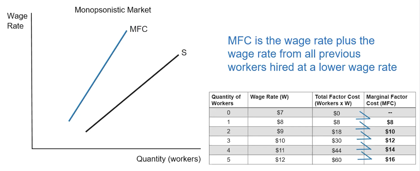
profit maximizing monopsony (optimal quantity of workers): MRC = MRP
MRP = demand
wage: intersection of supply and profit maximizing line (Q of workers)
vs a perfectly competitive market
monopsony graph is just pc market + MFC curve
pays lower wages + hires fewer workers
is not allocatively efficient and produces DWL