Chapter 4: The Market Forces of Supply and Demand

Importance of Market Forces and Graphs

• Significance of Chapter 4: This is considered the most important chapter in the textbook. Mastery of these concepts is essential for understanding all subsequent material in the book.

• Intensity and Length: This is one of the longest chapters and PowerPoint files, and it is the most graph-intensive section.

• Learning Curve: Students new to economics often struggle with the graphs, yet they are critically important to economics as a whole. An extra degree of study is explicitly encouraged.

Markets and Competition

• Market: A group of buyers and sellers of a particular product.

• Competitive Market: A market characterized by many buyers and many sellers, such that each individual has a negligible or minimal effect on the overall market price.

• Perfectly Competitive Market:

  • Defined by two primary characteristics:

    1. All goods offered for sale are exactly the same (homogeneous).

    2. Buyers and sellers are so numerous that no single participant can affect the market price.

  • Price Takers: In a perfectly competitive market, participants must accept the price determined by the market.

• Real-World Application: Perfectly competitive markets are relatively rare in reality. Most goods (like ice cream) come in many varieties, and many markets have few enough firms that some can influence the price.

• Utility of the Model: Even though it lacks perfect realism, the perfectly competitive model is used for instructive reasons. It makes learning easier and provides a foundation for analyzing more complex, imperfectly competitive markets.

The Theory of Demand

• Origin: Demand is driven by the behavior of buyers.

• Quantity Demanded ($QD$): The specific amount of a good that buyers are willing and able to purchase at a given price.

• Law of Demand: The claim that the quantity demanded of a good falls when the price of that good rises, provided all other factors remain constant.

• Ceteris Paribus: A Latin phrase meaning "other things being equal." This principle is fundamental to economic modeling.

• Intuition: As consumers, if a product becomes more expensive, we are less likely to want it; if it becomes cheaper, we want more of it.

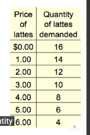
• Demand Schedule: A table illustrating the relationship between the price of a good and the quantity demanded.

• Helen’s Demand Example:

  • At a price of $0$, Helen demands more lattes.

  • At a price of $6$, she demands fewer.

  • Graphically, this inverse relationship (price up, quantity down) results in a downward-sloping demand curve.

  • The vertical axis represents Price ($P$) and the horizontal axis represents Quantity ($Q$).

  • 

Individual vs. Market Demand

• Market Quantity Demanded: The sum of the quantities demanded by all buyers in the market at each specific price.

• Aggregating Demand: To find the market demand curve, horizontal summation is used (x axis), adding together the individual quantities at every price level.

• The Two-Buyer Example (6:14):

  • Suppose the market consists only of Helen and Ken.

  • At $0$, the market quantity is $24$ (sum of their individual demands).

  • At $6$, the market quantity is $6$.

  • Even if a market has two million buyers, the process remains the same (summing all quantities), though it is more difficult to graph.

Demand Curve Shifters (Non-Price Determinants)

Variables other than the product's own price (taste of bitter coffee) can shift the entire demand curve. These include:

• Number of Buyers: An increase in the number of buyers leads to an increase in quality demanded at every price, shifting the curve to the right.

• Income:

  • Normal Good: A good for which demand increases when income increases (positive relationship). Examples: electronics, steak dinners. (i got paid so i wanna buy a steak dinner)

  • Inferior Good: A good for which demand decreases when income increases (negative relationship). Example: Top Ramen noodles (as people earn more money, they tend to consume less inexpensive instant noodles). (im poor af so ill just buy something cheap to eat)

• Prices of Related Goods:

  • Substitutes: Two goods where an increase in the price of one leads to an increase in demand for the other. Examples: pizza and hamburgers, Coke and Pepsi, laptops and desktops, CDs and music downloads.

  • Complements: Two goods where an increase in the price of one leads to a decrease in demand for the other. Examples: computers and software, college tuition and textbooks, bagels and cream cheese, eggs and bacon. (if tuition was sky rocketed, less students so no textbook demand)

• Tastes: Subjective preferences. Marketing (consumer behavior) focuses heavily on this. Example: The Atkins diet in the 1990s increased demand for eggs due to its emphasis on protein.

• Expectations: Expectations about the future (e.g., expecting a higher income tomorrow or worrying about job security) can change current buying habits.

The Theory of Supply

• Origin: Supply is driven by the behavior of sellers.

• Quantity Supplied ($QS$): The amount of a good that sellers are willing and able to sell.

• Law of Supply: The claim that the quantity supplied of a good rises when the price of the good rises, ceteris paribus.

• Sellers’ Perspective: Suppliers want higher prices to generate more revenue and profit; thus, higher prices incentivize more production.

• Supply Schedule: A table showing the relationship between price and quantity supplied.

  

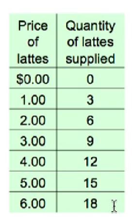
• Starbucks’ Supply Example:

  • At $0$, they supply $0$ lattes.

  • At $6$, they are willing to supply $18$ lattes.

  • This positive relationship (price up, quantity up) results in an upward-sloping supply curve.

Individual vs. Market Supply

• Market Quantity Supplied: The sum of quantities supplied by all sellers at each price.

• The Two-Seller Example:

  • Suppose the market consists only of Starbucks and Peet's.

  • At $1$, Starbucks supplies $3$ and Peet's supplies $2$, totaling a market supply of $5$.

  • At $6$, Starbucks supplies $18$ and Peet's supplies $12$, totaling a market supply of $30$.

Supply Curve Shifters (Non-Price Determinants)

Changes in these factors shift the entire supply curve rather than moving along it:

• Input Prices: The costs of production (e.g., wages, prices of raw materials like milk or coffee beans).

  • If input prices fall, production becomes more profitable, and sellers are willing to supply more at any given price (rightward shift).

  • If input prices rise, the curve shifts to the left.

• Technology: Determines how many inputs are required to produce a unit of output. Cost-saving technological improvements (like a more efficient latte machine) decrease production costs and shift the supply curve to the right.

• Number of Sellers: An increase in the number of sellers increases the market quantity supplied at each price, shifting the curve to the right (increased competition).

• Expectations: Sellers may adjust current supply based on future price expectations.

  • Example: If Texas oil producers expect oil prices to rise in the future, they may reduce supply now and store inventory to sell later at a higher price (leftward shift in current supply).

Market Equilibrium: Supply and Demand Together

• Equilibrium: The point where price has reached a level where quantity supplied equals quantity demanded ($QS = QD$). (Makes an X and crosses - where it crosses)

• Equilibrium Price ($P^*$): The specific price that equates quantity supplied and demanded (the point where the curves intersect). (ppl who want lattes meet ppl who sell lattes)

• Equilibrium Quantity ($Q^*$): The amount supplied and demanded at the equilibrium price.

• Latte Example: In the simplified model, equilibrium occurs at a price of $3$ and a quantity of $15$ lattes.

Market Disequilibrium: Surpluses and Shortages

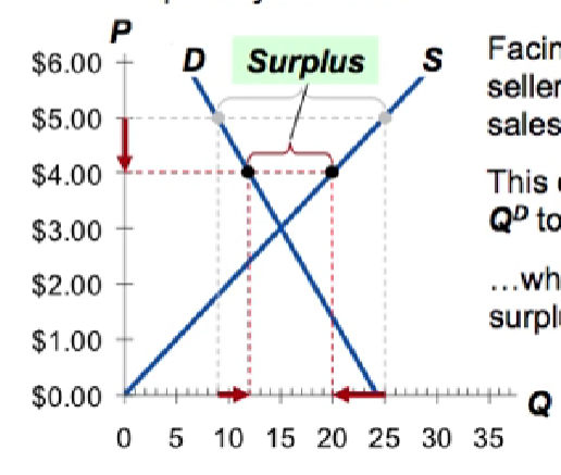
• Surplus (Excess Supply): Occurs when quantity supplied is greater than quantity demanded.

  • Example: At a price of $5$, suppliers produce $25$ lattes but consumers only want $9$, resulting in a surplus of $16$.

  • Response: Sellers cut prices to clear excess inventory, causing $QD$ to rise and $QS$ to fall until reaching equilibrium ($3$).

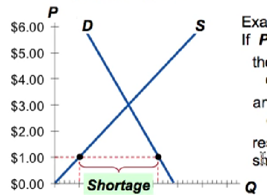
• Shortage (Excess Demand): Occurs when quantity demanded is greater than quantity supplied.

  • Example: At a price of $1$, consumers want $21$ lattes but sellers only provide $5$, resulting in a shortage of $16$.

  • Response: Sellers raise prices due to high demand, causing $QD$ to fall and $QS$ to rise until reaching equilibrium ($3$).

  • 

Three Steps for Analyzing Changes in Equilibrium

1. Shift Determination: Decide whether the event shifts the supply curve, the demand curve, or both.

2. Direction: Determine which direction the curve(s) shift (right/positive or left/negative).

3. Graphic Analysis: Use the supply and demand diagram to see how the shift changes the equilibrium price and quantity.

Case Studies: The Hybrid Car Market

• Scenario 1: Rising Gas Prices:

  • Gas is a complement to gasoline cars and a substitute for hybrids. Demand for hybrids shifts right ($D1 → D2$).

  • Result: Both equilibrium price and quantity increase. Note: There is a movement along the supply curve due to the price increase, but no shift in the supply curve itself.

• Scenario 2: New Production Technology:

  • Reduces production costs for hybrid producers. Supply curve shifts right ($S1 → S2$).

  • Result: Price falls, and equilibrium quantity increases.

• Scenario 3: Simultaneous Shifts (Rising Gas Price + New Technology):

  • Both demand and supply shift to the right.

  • Outcome: Equilibrium quantity definitely increases.

  • Ambiguity: The effect on price is ambiguous.

    • If demand increases more than supply, price rises.

    • If supply increases more than demand, price falls.

    • If they increase equally, price may stay the same.

Terminology: Shift vs. Movement

• Rule of Thumb: If the variable causing the change is on one of the axes (Price), you move along the curve. If the variable is not on an axis, the curve shifts.

• Change in Supply: A shift of the supply curve (due to input prices, technology, etc.).

• Change in Quantity Supplied: Movement along a fixed supply curve (due to a change in the product's price).

• Change in Demand: A shift of the demand curve (due to income, tastes, etc.).

• Change in Quantity Demanded: Movement along a fixed demand curve (due to a change in the product's price).

Questions & Discussion

• Q: Does this rule of thumb apply globally in economics?

• A: This rule (on-axis move vs. off-axis shift) works for most curves in economics, such as the supply curve, marginal cost curve, and IS/LM curves. However, it does not apply to Time Series graphs.

• Q: What about competition between tax software and professional preparers?

• A: If professional preparers (CPAs) raise their prices, this shifts the demand for tax software (the substitute) to the right. It does not shift the supply curve of the software directly.

Conclusion: Prices as Resource Allocators

• In market economies, prices are the signals that guide economic decisions. They adjust to balance supply and demand and are used to allocate scarce resources (time, money, materials) to their most valued uses. Markets are generally a superior way to organize economic activity.