2: Economic Theories, Data and Graphs
Statements
Positive statement: fact-based
Normative statement: opinion-based
PPB: As changes occur, the model must adapt and change.
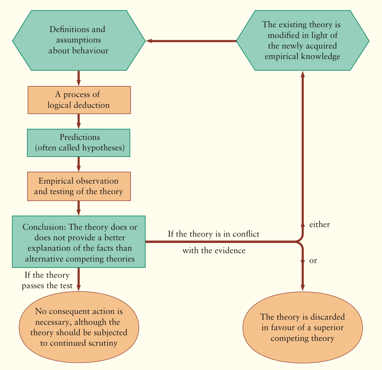
Economic Theories
Theories: constructed to explain things. Establish the relationship between economic variables. Hypotheses can be tested from the model.
e.g. the inverse relationship between price and demand.
Positive relations: both go up and follow each other directly.
Negative relations: inverse proportionality.
Variables
Variable: a well-defined item, such as a price or quantity, that can take on different positive values.
e.g. quantity of eggs may be defined as cartons of 12 grade A large eggs.
Variable prices of eggs is the amount of money that must be given up to purchase one of these cartons.
Endogenous variable: a variable where its value is determined within the theory. The theory is designed to explain them. → always on the y-axis as the dependent variable.
Exogenous variable: influences the endogenous variables but itself is determined outside of the theory, e.g. the state of weather and its impact upon the egg farm. The state of weather is not influenced by the egg market, but the price and quantity can be. (exo, outside.) → always on the x-axis as the independent variable.
Assumptions
A theory’s assumptions concern motives, directions of causations and the conditions where the theory is intended to apply.
Relationship: positive, negative, multiplicative, divisive.
Motives: Free-markets assume that people pursue their own self-interest when making decisions. — why an entity does something.
Direction of Causation: the assumption that one variable is related to another, assuming some kind of casual link between two variables, e.g., the weather and the supply of eggs. Producers supply more because of improved conditions. (rain → wheat.)
Conditions of application: assumptions are used to specify the conditions under which a theory is meant to hold. “No government” doesn’t mean anarchy, but rather a situation where government doesn’t significantly affect the studied situation.
Assumptions can be considered unrealistic, for instance, the extreme self-interest where the only economic motivator is complete maximization of profits. But, in considering the assumption, if profit is a key motivator, the model is substantially true.
Predictions
Hypotheses are propositions that can be deduced from a theory.
e.g. running out of oil. That was two variables: a divisive prediction.
Live modelling doesn’t work — e.g. markets will exhibit different behaviours when being observed by models. Test theories with only past data.
Theories are tested by contrasting predictions against empirical evidence.
Theories must be tested; therefore models must be built. e.g. aircraft testing. Models must subsequently be tested and pushed past limits, to determine its validity.
e.g. Boeing 737 MAX aircraft — in theory, models may work. But it doesn’t guarantee its validity when applied to real situations. Generally, it should be correct. There should be a degree of error expected.
Statistical Analysis
Correlation vs Causation
Correlation: a pattern exists between two things.
Causation: a cause-and-effect relationship.
Economic predictions generally involve casuality. Economists must take steps to differentiate between the two. Correlation can be applied to establish that a dataset is consistent with theory.
Mean: the average. sum / number
e.g. average condo prices: $450,000. But this includes luxury prices, many different types of apartments.
Median: the middle number
e.g. median house prices in Calgary, $1,000,000.
Mode: the most frequent number.
Have to qualify where data is from and know where your data is from & what it means.
Economic Data
Real world observations are used to test theories.
Recorded observations that are qualitative/quantitative of a set of variables.
Index Numbers
Index number: a measure of some variable, conventionally expressed as relative to a base period (which is considered to be 100.)
Calculating index number: [absolute value in a period] / [absolute value in base period] * 100
An index of 122.5 means that output is 22.5% greater than the base period.
When comparing an index number across non-base years, percentage change is not given by the absolute difference in value of the index number. To determine a percentage increase, [difference] / original.
Consumer Price Index: a price index of the average price paid by consumers for the typical collection of goods and services that they buy. It is derived from the weighed average of separate price indexes, weighed relative to average importance to a consumer.
e.g. subprime prices in the 2008 financial crisis; need some kind of reference point.
Examples of fuel price index numbers
Year | Price/litre | Index |
2021 | 1.15 | 1.15 / 1.10 × 100 =104.545 |
2022 | 1.10 | 1.10 / 1.10 × 100 =100 |
2023 | 1.12 | 1.12 / 1.10 × 100 =101.818 |
2024 | 1.18 | 1.18 / 1.10 × 100 =107.273 |
2025 | 1.24 | 1.24 / 1.10 × 100 =112.727 |
Pick a base year: 2022.
obs/base * 100
In 2021, fuel was 4.54% higher than in 2022.
Y1 - Y0 / Y0 to determine change between years.
Graphing Economic Data
Cross-Sectional Data: a number of different observations on one variable all taken in different places at the same timepoint.
Time-series data: Observations of one variable at successive points in time.
Scatter Diagrams: different variables on the x-axis and y-axis.
Data & lines of best fit can be presented linearly or with a non-linear function. e.g. with height, non-linear models are better.
Straight-line modelling is applied in this course.
Marginal change: slight changes in the slope (refer to Calc 1 at this point. Christ.)
Increasing marginal response: where the first derivative is positive.
Decreasing marginal change: where the first derivative is negative.
Cartesian Planes
Two-real number lines intersecting; plots (x,y)
Always apply quadrant 1; might also use quadrant 4.
x: exogenous variable
y: endogenous variable.
45 degree: 1:1 slope.
22.5 degree: 1:2 slope.
When a model is imposed on a dataset, we are imposing linearity on the data. Extrapolate the graph.
Linear Functions
y = b ± mx
Endogenous variable is always y.
Exogenous variable is always x.
The y-intercept will always stand alone as a 0th degree term. → constant term/autonomous term
Slope, also known as propensity (tendency for rise/run); the induced component.
Opportunity cost: the slope of the function.
For slope, care not to transpose observations.