integration

National School of Autonomous Systems

Analysis II First year

2023/2024

Chapter2:Integration

Riemann Integral

Definition. Let a and b be two real numbers such that a < B

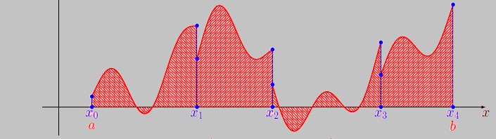
•subdivision: A subdivision of the closed bounded interval [a,b] is a finite family of real numbers

(x₀,x₁,...,x_n) such that a = x₀ < x₁ < ... < b = x_n. • The step of such a subdivision is the number

σ = max |x_k − x_k−₁|

1≤k≤n

In other words, it is the length of the largest interval in the subdivision of [a,b].”

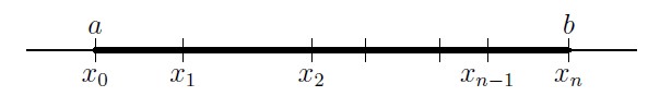
• The equidistributed: subdivision arises from a equidistant partitioning of [a,b] into n intervals of equal length. The points of the subdivision are given by(They are distributed according to an arithmetic progression with a common difference σ).

Definition (Riemann Sum) Let f be a function defined on [a,b], σ = (x₀,...,x_n) a subdivision of [a,b], and ∆ = (δ₁,...,δ_n) a set of real numbers such that for all k ∈ {1,...,n}, δ_k ∈ [x_k−1,x_k] (we say that the set ∆ is adapted to the subdivision σ).

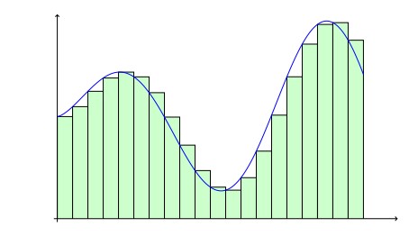
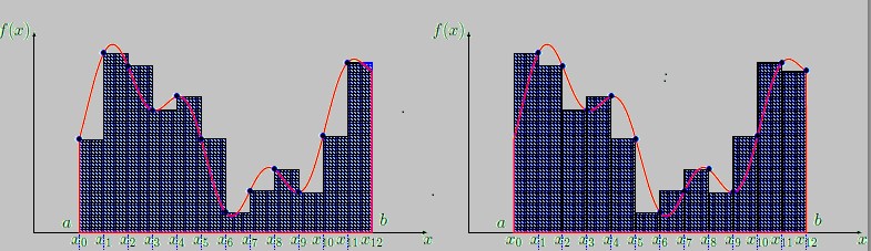
The Riemann sum of the function f associated with σ and ∆ is the number

n

S(f,σ,∆) = ^X(x_k − x_x−₁)f(δ_k).

k=1

This number represents the area of the union of rectangles with bases [x_k−1,x_k] and heights f(δ_k).

Example. Consider an equidistributed subdivision with

The corresponding Riemann sums are written as

Definition. (Riemann Integral) Let f : [a,b] → R be a bounded function. If there exists a real number l such that for every ε > 0, there exists α > 0 such that for every subdivision σ with steps < α for any subdivision adapted to σ, we have

|S(f,σ,∆) − l| < ε

we say that the function f is integrable (in the sense of Riemann) over [a,b] and the number l is the

integral of f over [a,b]. This number is denoted.

In other words, a function is integrable if and only if all its sequences of Riemann sums whose subdivision steps tend towards 0, are convergent with the same finite limit.

Remark.

• The variable used in the integral notation is called dummy

Z b

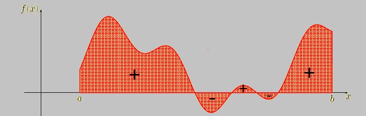
• The number f represents the algebraic area between the curve f and the x-axis, counting

a

negatively the parts below the axis and positively the parts above.

Theorem.

Let

f

beacontinuousfunctionontheinterval[

a,b

]

.Weperformasubdivisionof

[

a,b

]

witha

constantstepsize

h

(

h

=

b

−

a

n

.Let

)

k

∈

[0

,n

−

1]

,wedefine

x

k

=

a

+

k

b

−

a

n

=

a

+

kh

and

R

n

=

b

−

a

n

n

−

1

X

k

=0

f

(

x

k

)

,I

=

Z

b

a

f

(

x

)

dx

Wehavetheestimation

|

I

−

R

n

|≤

M

(

b

−

a

)

2

2

n

,M>

0

Thus,

lim

n

→∞

R

n

=

I

For the interval [0,1], we have

Proposition. Let f be a continuous function on [0,1], we define the sequences

and

We have

Definition. We say that a function f : [a,b] → R is piecewise continuous on the interval [a,b] if there exists a partition (x_i) (a = x₀ < x₁ < ... < x_n = b) of [a,b] such that for every i ∈ {0,...,n − 1}, the restriction of f to ]x_i,x_i+1[ is continuous and has finite limits at x_i and x_i+1 (meaning the restriction of f can be continuously extended over [x_i,x_i+1]).

Such a partition is called adapted to the piecewise continuous function f.

Proposition.

• Any continuous function on [a,b] is integrable on [a,b].
• More generally, any piecewise continuous function on [a,b] is integrable. Let x₁,x₂,...,x_n be its points of discontinuity, denote f^˜_k the extension of f at these points, then

Properties Let f,g : [a,b] be two integrable functions and α,β ∈ R, we have

Z Z Z

i) b^af(x)dx = − a^bf(x)dx and a^af(x)dx = 0.

Z Z Z ii) a^bf(x)dx = a^cf(x)dx + c^bf(x)dx for all c ∈ [a,b].

Z Z Z

• 1. a^b(αf + βg)(x)dx = α a^bf(x)dx + β a^bg(x)dx.

Z b

• 1. If f(x) ≥ 0 on [a,b] then f(x)dx ≥ 0. and f ≥ g on [a,b],then

a v) .

• 1. If f is even on [−a,a] then
  2. If f is odd on [−a,a] then.

Example.

We want to compute using Riemann integral i.e

in the following cases

• 1. Let f(x) = λ (constant function), we have

) ( area of a rectangle).

• 1. f(x) = x, we have

.

• 1. f(x) = e^x, we have

.

We can also use Riemann integral to compute some sum of numerical series.

Example. Calculate the limits of the following sequences

We write

thus, we only need to take f(x) = x which is continuous on [0,1]. We have

.

Similarly for the sequence (v_n), we have

We take the function f(x) = cosx which is continuous on the interval [0,], thus

Primitive and Integral of a Continuous Function

Definition.

• If f is a continuous function on I, a primitive of f is any differentiable function on I into R whose derivative is equal to f.
• If F is a primitive of f (f a continuous function), meaning F⁰ = f, then the primitives of f on I are functions F + λ, λ ∈ R.

Theorem.

Suppose

f

isacontinuousfunctionon

I

into

R

and

a,b

∈

I

.If

F

isaprimitiveof

f

on

I

,then

Z

b

a

f

(

x

)

dx

=

F

(

b

)

−

F

(

a

)

.

Corollary.

If

f

∈C

1

(

I

)

and

x,a

∈

I

,then

Integration by Parts

Theorem.

If

u

and

v

aretwo

C

1

functionson[

a,b

]

,wehave

Z

b

a

u

(

x

)

v

0

(

x

)

dx

=

u

(

x

)

v

(

x

)

b

a

−

Z

b

a

u

0

(

x

)

v

(

x

)

dx

Proof. If u,v ∈ C¹([a,b]), then uv ∈ C¹([a,b]) and we have

On the other hand, we have

Hence the result.

Remark. In the case of an indefinite integral, integration by parts is written as

Z Z

u(x)v⁰(x)dx = u(x)v(x) − u⁰(x)v(x)dx.

Example. We want to compute, by integration by parts, the following integrals

Z Z Z

I₁ = arctan(x)dx; I₂ = arccos²(x)dx; I₃ = sin(2x)ln(tan(x))dx

1-For I₁, we set

I₁ becomes

2-We set

I₂ becomes

We apply integration by parts again, setting

Then we have

I₂ = xarccos²(x) − ^p1 − x² arccos(x) − x + C, C ∈ R.

For I₃, we set

Then we have

Example. Let I_n be the Wallis integral, given by

By setting

we get

which gives us the relation

I_n = (n − 1)I_n−₂ − (n − 1)I_n

Thus, we have the following recurrence relation

Similarly, we have

.

• For n = 2p, we have

• For n = 2p + 1, we have

where

and

thus

and

Change of Variable

Proposition.

Let

f

beacontinuousfunctionfrom

I

to

R

and

φ

a

C

1

functionfrom

J

to

I

.If

α,β

∈

J

,then

Z

φ

(

β

)

φ

(

α

)

f

(

x

)

dx

=

Z

β

α

f

(

φ

(

t

))

φ

0

(

t

)

dt

By definition, the transformation x = φ(t) (t ∈ J) is called a change of variable.

Proof. f is a continuous function on I, thus it has a primitive F, and we have

Since the function F ◦ φ is a C¹ function (composed of two C¹ functions), we have

Example. Calculate the following integrals

• For I₁, we let t = x², then dt = 2xdx, thus

.

• For the integral I₂, we let t = cosx, then dt = −sin(x)dx and We obtain

.

Primitive of a Rational Fraction

1- Rational fraction of the first kind: Let (a,b) ∈ R^? × R and k ∈ N^?, a rational fraction of the first kind is any fraction of the form

Its integral is given by

2-Second species rational fraction: Let (a,b,c) ∈ R^∗ × R² and k ∈ N^∗, we call a second species rational fraction any fraction of the form

with ∆ = b² − 4ac < 0.

To integrate this fraction, we first write the numerator as a function of the derivative of ax² +bx+c, we have So

Let

and

For the calculation of the integral I_k, it’s direct, we have

For J_k, we write ax² + bx + c in its canonical form, we have

with.

We make the change of variable is written as

If k = 1, we have

If k ≥ 1, we will find a recurrence formula between J_k and J_k+1, using integration by parts. Example. We want to calculate the integral

here we have ∆ < 0, it’s a second species rational fraction. We write

Let, we write

Let, we obtain

To calculate this integral, we will integrate by parts the function , by setting

So

Finally, we have

The integral I is given by

.

3. Any rational fraction: Let P and Q be two polynomials, we define the rational fraction

The aim here is to write F in the form of the sum of rational fractions of the first and second species, in order to be able to integrate it. For that, we have the following steps

• Step 1: Simplify F (look for common elements between P and Q).
• Step 2: If degP ≥ degQ, we perform the Euclidean division. We write

such that degR < degQ

• Step 3: Factorize the denominator, for example, we have

Q(x) = (x − a₁)(x − a₂)² + (x − x₃)³(α₁x² + β₁x + γ₁)(α₂x² + β₂x + γ₂)²

such that 0 and

• Step 4: Decompose the fraction into simple elements, we have

Example. Calculate the following integrals

1- We will first decompose the rational fraction into simple elements. The fraction is already simplified and the degree of the numerator is strictly less than the degree of the numerator, so we go directly to step 3. We have x³ − 7x + 6 = (x − 1)(x − 2)(x + 3), then

a,b,c ∈ R constants to be determined. We can do it by identification, or we have

(?)

• To determine a, we multiply (?) by (x − 1), then we put x = 1. We have

• To determine b, we multiply (?) by (x − 2), then we put x = 2. We have

• To determine c, we multiply (?) by (x + 3), then we put x = −3. We have

So

.

2-Let the rational fraction here the degree of the numerator is greater than

the degree of the denominator, so we perform the Euclidean division

We have x⁴ − 2x³ + 2x − 1 = (x − 1)³(x + 1), so

with

We write

(??)

Now we determine the constant c, we have

For b it suffices to give a value to x in (??), we take for example x = 0, we obtain . The

decomposition into simple elements of our fraction is written

.

Consequently, we obtain

.

Integrals Reducible to Rational Fraction Integrals

Throughout, R will denote a rational function.

1. Integrals of Rational Functions in e^x These are integrals of the form ^R R(e^x)dx, where we perform the variable change t = e^x, giving .

Example.

.

We have

We write

.

So

For c, we have

and for d we just need to give a value to x, we find d = −2. Thus

1. Rational Functions in cosx and sinx: These are integrals of the form ^R R(cosx,sinx)dx. We use the variable change), giving

Example. We want to calculate the integral.

We set), obtaining the integral

This variable change always works but sometimes the calculation is long. There are special cases where we can avoid this change of variable.

• • If our integral is of the form ^R R(sinx)cosxdx, we set t = sinx, dt = cosxdx. Example.

• • If our integral is of the form ^R R(cosx)sinxdx, we set t = cosx, dt = −sinxdx. Example.

• • If our integral is of the form ^R R(tanx)dx or ^R R(sinx,cosx)dx where cosx and sinx appear only with even powers, we set t = tanx and we have the formulas

Example.

Z

Bioche’s Rule: In the case of an integral of a fraction R(x)dx dependent on sinx, cosx and tanx , we can also use Bioche’s rule which serves to give the appropriate variable change. We set

ω(x) = R(x)dx

We distinguish the following four cases

• 1. First case: If ω(−x) = ω(x) (invariant with respect to −x), we perform the variable change t = cosx.
  2. Second case: If ω(π − x) = ω(x) (invariant with respect to π − x), we perform the variable change t = sinx.
  3. Third case: If ω(π + x) = ω(x) (invariant with respect to π + x), we perform the variable change t = tanx.
  4. Fourth case: If none of the above properties hold, we opt for the variable change

Example.

1. Consider the integral. We set

we have

) (the variable change t = cosx doesn’t work).

) (the variable change t = sinx doesn’t work).

) (the variable change t = tanx works).

Indeed, we have

Thus

1. Calculate the integral. By taking: , we have ω(x) =

ω(−x), so we set t = cosx. The integral I becomes

3. Rational Functions in coshx and sinhx: These are integrals of the form ^R R(coshx,sinh)dx.

We use the variable change) and the formulas

Example.

Special case.

Z

1. R(coshx)sinhxdx, we set t = coshx.

Example.

Z

1. R(sinhx)coshxdx, we set t = sinhx.

Example.

Z Z

1. R(tanhx)dx or R(coshx,sinhx)dx where sinhx and coshx only appear with even powers, we set t = thx and we use the formulas

Example.

argth(argth

Remark. As coshx and sinhx are expressed as functions of e^x, we can therefore reduce to the case of an integral of a rational function in e^x and use the change of variable t = e^x.

Example. Consider the integral. We have

,

we obtain

Abelian integrals:

• Integrals of the form

the recommended change of variable is.

Example Compute the integral

.

We set and We get

I = −2argth(t) + 2arctan(t) + C = −2argth

Z

• Integrals of the form R(x,^pax² + bx + c)dx. By writing ax²+x+c in canonical form, this integral is reduced to the following cases

Z

• 1. R(t,^p1 − t²)dt, we set t = sinu, t = cosu.

Z

• 1. R(t,^p1 + t²)dt, we set t = sinhu.

Z

i) R(t,^pt² − 1)dt, we set t = coshu.

Example. Calculate the integral.

We have

We set, we obtain

th(

I

2

=

Z

dt

(

√

3

t

−

1)

√

t

2

+1

=2

Z

ch

udu

ch

u

(

√

3

sh

u

−

1)

2

=

du

(

√

3

sh

u

−

1)

=

2

Z

1

√

3(

2

s

1

−

s

2

)

−

1

2

ds

1

−

s

2

4

=

Z

ds

s

2

+2

√

3

s

−

1

=

Z

1

s

+

√

3

−

2

ds

−

Z

1

s

+

√

3+2

ds

=

ln

s

+

√

3

−

2

s

+

√

3

−

2

+

C

ln

=

th(

argsh

(

t

)

2

)+

√

3

−

2

th(

argsh

(

t

)

2

)+

√

3

−

2

+

C

=

ln

th(

argsh

(

2

x

+1

√

3

)

2

)+

√

3

−

2

argsh

(

2

x

+1

√

3

)

2

)+

√

3

−

2

+

C

(we set t = shu then .

Other types of integrals

Z

• Let I = e^αxP(x)dx where α ∈ R and P is a polynomial of degree n (n ∈ N^?). We proceed with

n successive integration by parts and we find that the primitives are of the form e^αxQ(x) where Q is a polynomial of the same degree as P, which suggests another calculation method namely setting

I = e^αxQ(x) + C, derive I to calculate Q. Thus

(e^αxQ(x))⁰ = e^αxP(x) = αe^αxQ(x) + e^αxQ⁰(x)

so

P(x) = αQ(x) + Q⁰(x)

which gives the coefficients of Q by simple identification.

Z

Example. I = (x² + 1)e^xdx = (ax² + bx + c)e^x + C with a, b, c verifying

x² + 1 = ax² + bx + c + 2ax + b = ax² + (b + 2a)x + c

thus by identification a = 1, b = −2 and c = 1, we find I = (x² −2x+1)e^x +C = e^x(x² −2x+1)+C.

Z

• sin^m xcosⁿ xdx such that m, n ∈ Z. We have the following cases
  1. If m is odd and positive, do the change of variable t = cosx.
  2. If nis odd and positive, do the change of variable t = sinx.
  3. If m and n even and postives, use the formulas

Z

• sin(ax)sin(bx)dx −→ use the formula sin(

Z

• sin(ax)cos(bx)dx −→ use the formula sin(

Z

• cos(ax)cos(bx)dx −→ use the formula cos(