AP Macro Unit 3 Notes: National Income and Price
Unit Three: National Income and Price Concepts
Key Concepts
1. Multipliers
Definition: Economic concept that measures the effect of initial spending on overall GDP as it ripples through the economy.
Key components:
Disposable Income: Personal income minus taxes.
Consumers have two choices for disposable income: spend or save.
Marginal Propensity to Consume (MPC)
Definition: Percentage of new income that a consumer is likely to spend.
Can be expressed as a decimal. Example:
If disposable income increases by $1,000:
Spending increases by $800 → MPC = 0.8 (or 80%)
Savings increases by $200 → MPS = 0.2 (or 20%)
Marginal Propensity to Save (MPS)
Definition: Percentage of new disposable income that a consumer saves rather than spends.
Connection: MPC + MPS = 1
Example of Spending Ripple Effect
Initial spending: $800 on a fishing boat.
Boat store owner now has:
New disposable income: $800
Spend 80% ($640) → Buys a new bicycle
Bicycle store owner then spends 80% of $640… and so on.
Example expenditure sequence:
Boat → Bicycle → Television → Trip → Gym Membership
Continuous spending leads to a larger impact on GDP.
2. Spending Multiplier
Formula:
Example Calculation:
Given MPS = 0.2 →
Economic impact of increased consumption:
Initial spending of $800 can result in a $4,000 increase in GDP.
3. Tax Multiplier
Definition: Evaluates the impact of tax changes on overall disposable income and therefore GDP.
Formula:
Absolute value of tax multiplier is one less than spending multiplier.
Example Calculation:
Given MPC = 0.8 and MPS = 0.2:
Implication of tax reduction:
A decrease of $10 million in taxes could lead to a maximum of $40 million increase in GDP.
ASAD Model of the Economy
1. Aggregate Demand Curve
Definition: Represents the total demand for all goods and services in the economy.
Graphical Representation: Price level y-axis, Real GDP x-axis.
Shape: Downward sloping, indicating an inverse relationship between price level and output.
Reasons for Downward Sloping Aggregate Demand Curve
Wealth Effect: As prices fall, real wealth increases, leading to increased purchasing.
Interest Rate Effect: Lower price levels lead to lower interest rates and higher investment.
Net Export Effect: At lower prices, exports become cheaper, increasing demand from foreign countries.
2. Shifters of Aggregate Demand
Four main components affecting aggregate demand (represented as C + IG + G + XN):
Consumer Spending (C)
Gross Investment (IG)
Government Purchases (G)
Net Exports (XN)
Impact on Curve: An increase in any of the components shifts the aggregate demand curve to the right; a decrease shifts it to the left.
3. Short-Run Aggregate Supply Curve (SRAS)
Represents total supply of goods and services within the economy in the short run.
Relationship: Direct—higher prices lead to higher output due to sticky wages and resource prices.
Direction of curve shifts:
Factors creating shifts in SRAS:
Resource Prices: Higher resource prices → left shift; Lower → right shift.
Productivity: Increase → right shift.
Inflation Expectations: Higher expectations → left shift; Lower expectations → right shift.
Business Taxes: Decrease in business taxes → right shift; Increase → left shift.
Business Regulations: Increase → left shift; Decrease → right shift.
4. Long-Run Aggregate Supply Curve (LRAS)
Characteristics: Vertical at the full employment level of output (denoted as YF).
Implication: Long run output is not affected by price levels as wages are flexible.
Represents long-standing potential output which can be influenced by various economic factors (resources, productivity, technology changes).
Shifts in LRAS:
Inward shift indicates reduced potential (e.g., natural disasters).
Outward shift indicates increased potential (e.g., technological advancements).
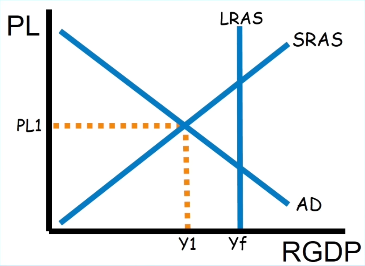
5. Equilibrium in ASAD Model
Short-run Equilibrium: Occurs at the intersection of AD and SRAS.
Inflationary Gap: When current output exceeds long-run potential (Y1 > YF), typically characterized by low unemployment.
Recessionary Gap: When current output is below long-run potential (Y1 < YF), indicating high unemployment and low national income.
Long-Run Equilibrium: The point where AD intersects LRAS; current output equals full employment output. Unemployment is at natural rate.
Shocks to the Economy
Demand Shocks: Increase in net exports leading to inflationary gap caused by increases in AD. Conversely, a decrease in consumer confidence leads to lower price levels—negative demand shock.
Supply Shocks: Changes in SRAS from external factors (e.g., oil prices affect production).
Positive shocks (e.g., drop in oil prices) can shift SRAS right, causing price levels to fall and output to increase—indicating an inflationary gap.
Negative shocks (e.g., external costs) can shift SRAS left, causing price levels to rise and output to decrease, associated with cost-push inflation (stagflation).
Long-term Adjustments to Equilibrium
Self-Correction without Intervention: In recessionary gap, lower wages lead SRAS back to equilibrium; in inflationary gap, rising wages shift SRAS left.
Fiscal Policy Adjustments
Expansionary Fiscal Policy: Used to combat unemployment by increasing government spending or reducing taxes, shifting AD to the right, restoring employment.
Contractionary Fiscal Policy: Used to address inflation by decreasing government spending or raising taxes, shifting AD left to return to equilibrium.
Automatic Stabilizers: Mechanisms that adjust based on business cycle changes, affecting budget deficits without active intervention (e.g., taxes and transfer payments) to mitigate economic fluctuations.Conclusion
Strong grasp of multipliers, ASAD model, various shifts, and their impact on GDP is essential.
Recommens.dation to explore additional resources and review materials for better exam preparedness.
Engagement reminder: Like and subscribe to support the channel and access extra study resource