Chapter 7: Pure Competition in the Short Run

Four Market Models

• Pure competition, Pure monopoly, Monopolistic competition, Oligopoly

• LO1 Market Structure Continuum: Pure Competition — Monopolistic Competition — Oligopoly — Pure Monopoly

• Key idea: different market structures vary in number of firms, product type, price-setting ability, entry barriers, nonprice competition, and typical examples.

• Pure competition

  • Very large number of firms

  • Standardized product

  • Price takers

  • Very easy entry and exit

  • Demand for an individual firm is perfectly elastic (horizontal); industry demand is downward-sloping

  • No nonprice competition

  • Examples: Agriculture

• Pure monopoly

  • One firm

  • Unique product; no close substitutes

  • Price setter; significant barriers to entry

  • Substantial nonprice competition may be present in advertising, branding, etc.

  • Example: Local utilities (illustrative)

• Monopolistic competition

  • Many firms

  • Differentiated products

  • Some price-setting ability within narrow limits

  • Relatively easy entry and some nonprice competition (advertising, branding)

  • Examples: Retail dresses, shoes

• Oligopoly

  • Few firms

  • Standardized or differentiated products

  • Price competition limited by mutual interdependence; tendency toward collusion

  • Significant nonprice competition and strategic behavior

  • Examples: Steel, autos, airlines

• Monopoly vs competition (summary): control over price, product differentiation, entry barriers, and strategic behavior differ across models.

Pure Competition: Characteristics (LO2)

• Very large numbers of independent sellers each acting alone cannot influence the market price by increasing or decreasing their output because each has such a tiny part of the entire market.

• A standardized product is a product for which all other products in the market are identical and thus are perfect substitutes. The consequence of this is that buyers are indifferent as to whom they buy from.

• Price takers have no pricing power; in other words, no ability to price their product.

• Easy entry and exit means that there are no obstacles to entry or to exit the industry.

• Perfectly elastic demand means that firm has no power to influence price so the firm merely chooses to produce a certain level of output at the price that is given.  The demand curve is not perfectly elastic for the industry; it only appears that way to the individual firm, since they must take the market price no matter what quantity they produce.  The firm faces a perfectly elastic demand because each individual firm makes up such a small part of the total market and the goods are perfect substitutes.  Note that this perfectly elastic demand curve is a horizontal line at the price.

Revenue Concepts: Average Revenue, Total Revenue, and Marginal Revenue (LO3)

• Average Revenue (AR) = TR / TQ = P

• Total Revenue (TR) = P × TQ

• Marginal Revenue (MR) = ΔTR / ΔTQ

• In perfect competition: P = AR = MR

• These relationships lead to the familiar condition for profit maximization in the short run: MR = MC (when producing)

• Relationship summary (LaTeX):

  • AR=TR/TQ=P

  • TR=PXTQ

  • MR=\Delta TR/\Delta TQ

  • In pure competition: P = AR = MR
    

When a firm charges the same price for each unit of output, the average revenue is just the price of the good.  Total revenue refers to the total amount of money that the firm collects for the sale of all of the units of their good.  Marginal revenue reflects the additional revenue that the firm will receive by producing one more unit of output. 

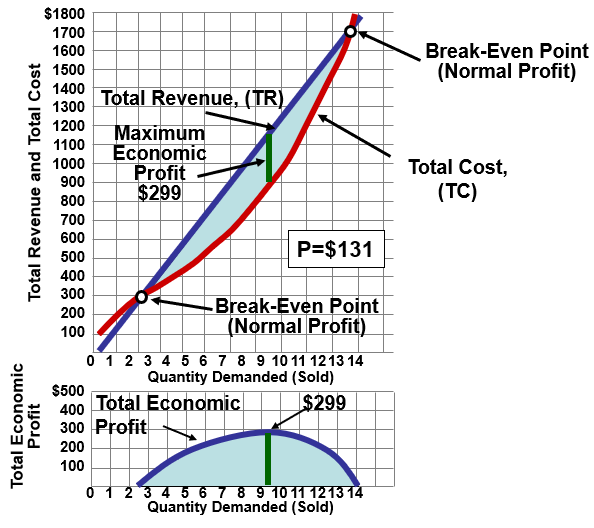
Short-Run Profit Maximization: TR–TC Approach (LO3)

• Three guiding questions:

  • What economic profit (or loss) will be realized?

  • If profitable, what amount?

  • Should the firm produce in the short run?

• Example data (Price = 131) – Total Revenue, Total Cost, and Profit by Output (Q)

  • For each Q from 0 to 10:

  • TR = TR=131XQ

  • TC and Profit (Profit = TR − TC) are given below.

  • Data:

  • Q = 0: TR = 0, TC = 100, Profit = -100

  • Q = 1: TR = 131, TC = 190, Profit = -59

  • Q = 2: TR = 262, TC = 270, Profit = -8

  • Q = 3: TR = 393, TC = 340, Profit = +53

  • Q = 4: TR = 524, TC = 400, Profit = +124

  • Q = 5: TR = 655, TC = 470, Profit = +185

  • Q = 6: TR = 786, TC = 550, Profit = +236

  • Q = 7: TR = 917, TC = 640, Profit = +277

  • Q = 8: TR = 1048, TC = 750, Profit = +298

  • Q = 9: TR = 1179, TC = 880, Profit = +299

  • Q = 10: TR = 1310, TC = 1030, Profit = +280

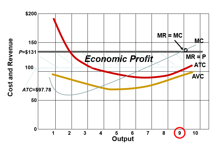
• Marginal Revenue–Marginal Cost (MR-MC) approach (Price = 131) – Output where MR = MC

  • Marginal Cost (MC) schedule (from data):

  • Q = 1: MC = 90

  • Q = 2: MC = 80

  • Q = 3: MC = 70

  • Q = 4: MC = 60

  • Q = 5: MC = 70

  • Q = 6: MC = 80

  • Q = 7: MC = 90

  • Q = 8: MC = 110

  • Q = 9: MC = 130

  • Q = 10: MC = 150

  • Price (MR) = 131, so the profit-maximizing output is where MC ≈ MR, i.e., Q = 9 (MC9 = 130 is just below MR; MC10 = 150 > MR).

  • Profit at Q = 9 (from TR–TC): TR - TC = 1179 - 880 = 299. (Matches the TR–TC table where Profit at Q = 9 is +299.)

  • At Q = 10, Profit = 280 (lower than at Q = 9), so Q = 9 is the MR = MC maximum in this dataset.

• Interpretation:

  • If P > ATC at the chosen Q, the firm earns positive economic profit; ATC at the profit-maximizing output (Q ≈ 9) is about 97.78 per unit (ATC at Q = 9). With P = 131, the firm earns profit because P > ATC.

  • The break-even point (where P × Q = TC) would occur where P equals ATC; in this dataset, ATC at the profit-maximizing output is well below P, so profits exist.

  • Rule: set MR = MC to find the quantity; compare price to ATC to determine profit status.

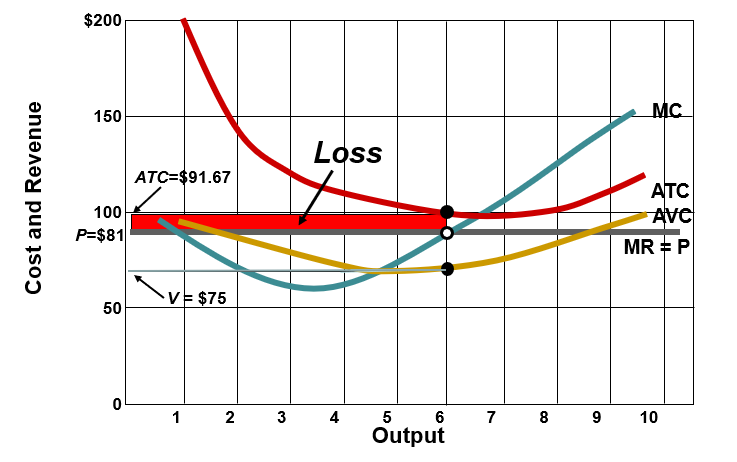
Loss-Minimizing Case: MR–MC Rule When P < ATC but P > AVC (LO3)

• Principle: If the firm must incur losses, it should still produce in the short run as long as price covers average variable costs (P ≥ AVC). If P < AVC, the firm should shut down.

• Case summary: When P < ATC but P > AVC, the firm produces at MR = MC to minimize losses (since fixed costs are sunk in the short run).

• Example data (P = 81; ATC = 91.67; AVC = 75):

  • The firm’s per-unit cost structure indicates that producing at the MR = MC output minimizes losses relative to permanent shutdown.

  • Loss equals total cost minus total revenue: Loss = TC − TR, with TC > TR when P < ATC.

  • In this example, AVC is $75 and MC schedule intersects MR near the output where MC ≈ 81, yielding a smaller loss than if the firm produced less or shut down. The key takeaway is the rule, not the exact numeric output: produce where MR = MC as long as P ≥ AVC; if P < AVC, shut down.

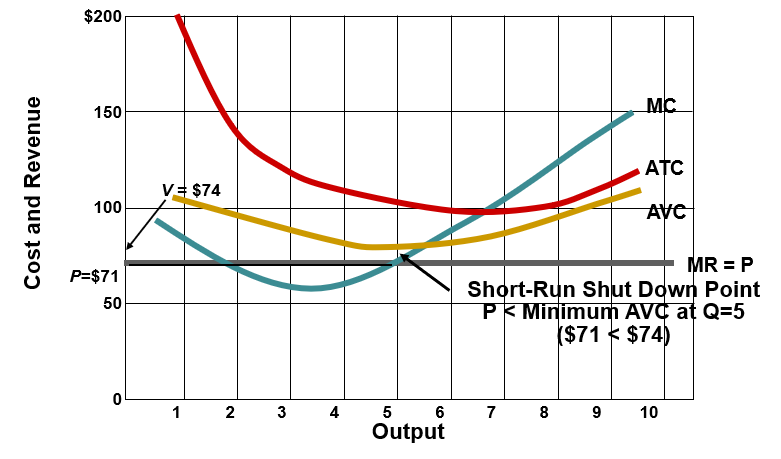
Shutdown Case: Sunk Costs and the Shutdown Rule (LO3)

• Sunk cost concept:

  • Sunk costs are past, unrecoverable costs and should be ignored when making current decisions.

  • In the short run, fixed costs are sunk costs for decision purposes.

  • Decision rule: compare price (P) to Average Variable Cost (AVC).

• Practical shutdown rule:

  • Stay open if P ≥ min AVC; shut down if P < min AVC.

• Example: Restaurant/off-season case

  • Fixed costs (e.g., fixed operating costs) may be irrelevant to the shutdown decision.

  • If lunch revenue ($500) < total variable costs ($1,000), then shut down for lunch; if revenue exceeds variable costs, continue operation even with other capacity idle.

• Short-run shutdown point (example):

  • Given a dataset where min AVC occurs at Q = 5 with AVC = 74, and a shutdown price is P = 71 (P < min AVC).

  • Therefore, the firm should shut down when the market price falls to or below $71 in that setup.

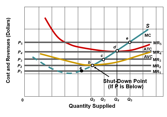
• Marginal cost and short-run supply relationship (LO4):

  • The short-run supply curve is the portion of the MC curve that lies above the minimum AVC.

  • At any price P above the shutdown price, the firm supplies the quantity where MC = MR = P.

  • Here is a generalized depiction of how the marginal cost curve becomes the short run supply curve. Examine the MC for the competitive firm.  If price is below AVC, then the firm should shut down and produce 0.  If the price is equal to or above AVC, the firm should produce.   The MC curve that is above the AVC curve becomes the short run supply curve.  The break-even point is point d where the firm earns a normal profit  because Price=ATC here.

Summary: Production Question (LO3)

• Should the firm produce in the short run?

  • Yes, produce where MR = MC:

  • If P > ATC, the firm is profitable (positive economic profit).

  • If P > min(AVC) but P < ATC, the firm incurs losses but covers a portion of fixed costs; it should continue producing to minimize losses.

  • If P < min(AVC), the firm should shut down (do not produce) because variable costs exceed revenue.

• In short-run terms:

  • Produce if MR = MC and either P > ATC (profit) or P > min(AVC) (avoid shutting down and minimize losses).

  • Shut down if P < min(AVC).

Firm and Industry: Equilibrium (LO4)

• Market supply vs. market demand (example with 1000 firms):

  • Individual firm supply is the portion of its MC curve above AVC.

  • Market supply is the sum of all firms’ supplies: S = ∑ S_i.

• A sample short-run schedule (illustrative data):

  • Price $151: Individual firm quantity supplied = 10; Total for 1000 firms = 10,000; Quantity demanded (Qd) = 4,000

  • Price $131: Individual firm quantity supplied = 9; Total supply = 9,000; Qd = 6,000

  • Price $111: Individual firm quantity supplied = 8; Total supply = 8,000; Qd = 8,000

  • Price $91: Individual firm quantity supplied = 7; Total supply = 7,000; Qd = 9,000

  • Price $81: Individual firm quantity supplied = 6; Total supply = 6,000; Qd = 11,000

  • Price $71: Individual firm quantity supplied = 0; Total supply = 0; Qd = 13,000

• Equilibrium in this example occurs where market supply equals market demand: at price $111 with total quantity supplied 8,000 and quantity demanded 8,000 (Q_eq = 8,000).

• Economic profit in equilibrium:

  • If price exceeds average total cost at the equilibrium output, firms earn profits; if price equals ATC, profits are zero (normal profit); if price is below ATC but above AVC, losses are incurred but may be minimized; long-run entry/exit would drive profits toward zero in a competitive market.

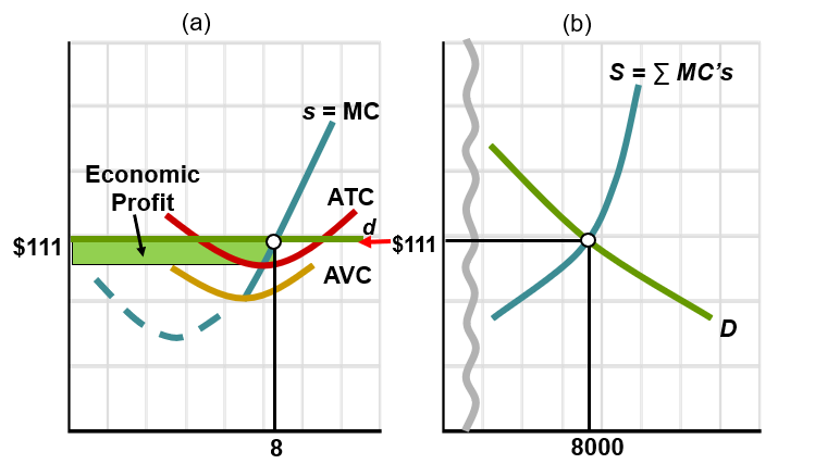
• Short-run competitive equilibrium for (a) a firm and (b) the industry.  The horizontal sum of the 1000 firms’ individual supply curves (s) determines the industry supply curve (S). Given industry demand (D), the short-run equilibrium price and output for the industry are $111 and 8000 units. Taking the equilibrium price as given, the individual firm establishes its profit-maximizing output at 8 units and, in this case, realizes the economic profit represented by the green area.

  
  Individual firms must take price as given, but the supply plans of all competitive producers as a group are a major determinant of product price.

Fixed Costs and Long-Run Perspective (Page 21)

• Shutting down in the short run does not imply shutting down forever; in the future, prices may recover.

• Some firms switch production on/off with market conditions (e.g., oil producers, resorts, off-season production).

• Fixed costs are irrelevant to the shutdown decision in the short run (they are sunk costs for this period).

• Practical implication: the presence of fixed costs can influence short-run decisions but does not dictate long-run market structure or entry/exit in the immediate term.

Quick Formulas to Remember

• AR = TR / TQ = P

• TR = P × TQ

• MR = ΔTR / ΔTQ

• In pure competition: P = AR = MR

• Profit (or loss) = TR − TC

• Shutdown condition: Shut down if P < min(AVC); otherwise produce where MR = MC

• Short-run supply: the MC curve above the minimum AVC

• Break-even condition (for a given Q): P = ATC at that Q

• Profit per unit at a given Q: P − ATC

• Total profit at a given Q: (P − ATC) × Q (when MR = MC and P > ATC)

Quick Connections to Real World and Concepts

• The four market structures frame how price, output, and profits respond to shifts in demand, costs, and entry/exit barriers.

• In a purely competitive short run, firms respond to price signals by adjusting output to the MR = MC rule; profits depend on how P compares to ATC.

• The shutdown rule demonstrates the separation between fixed costs (sunk in the short run) and variable costs (relevant for decision-making).

• The concept of industry supply being the sum of individual firm supplies emphasizes the importance of market structure for macro-level outcomes like equilibrium price and total production.