TM355 Communications Technology - Coexistence Part 3 Notes
Noise, Interference, and Coexistence
Introduction
Real-world communication systems are affected by noise and interference.
This part of Block 1 focuses on the effects of noise and interference in real-world communications.
It revisits theoretical concepts from Parts 1 and 2 to examine real-world differences.
The inverse fourth-power law is a model for radio wave propagation in urban environments, but other factors exist.
Digital modulation schemes and bit error rates are revisited, revealing that schemes with more symbols aren't always desirable due to noise.
There's a theoretical maximum data rate achievable in a noisy channel.
Spectrum management is a regulatory approach to reduce noise effects.
Overview of this part:
Section 2 introduces noise and interference and their causes.
Section 3 considers the urban environment and its challenges for mobile communications.
Sections 4-6 focus on noise and its effects:
Section 4: Signal-to-noise ratio.
Section 5: Theoretical limitations on data rate.
Section 6: Bit error rate (BER).
Section 7 introduces spectrum management.
Section 8 is the part summary.
Noise and Interference
Noise and interference affect real-world communication systems.
Examples of interference include:
Unwanted stations on AM or FM radio.
Mobile phones interfering with landline phones.
Domestic appliances or power tools causing crackling on the radio.
Natural sources of noise:
Electrical storms.
Solar flares emitting radiation and energetic particles, disrupting radio communications.
Auroras.
Noise generated within the receiver:
Receivers amplify signals, also amplifying electrical noise from components.
Distinction between noise and interference:
Noise: From natural sources, often unavoidable.
Interference: From unwanted transmissions.
Regulatory bodies develop and enforce policies to avoid interference.
Usage is regulated by licenses, but there are other alternatives.
Avoiding mutual interference between two radio transmitters:
Use different frequencies (e.g., different TV channels).
Separate transmitters geographically.
Time-division multiplexing.
Different antenna polarizations (horizontal and vertical).
Directional antennas.
Interference is a particular problem with radio due to its shared medium.
Noise and interference affect signals in copper cables.
Conductors can act as antennas.
Low-frequency energy from mains supply can cause 'hum'.
Electromagnetic compatibility (EMC) mitigates interference:
Emissions limits: Limits on power radiated at different frequencies.
Immunity standards: Devices must function normally in the presence of radio waves.
Legal restrictions limit radiated power for both wanted and unwanted transmissions.
Mobility and urban environments
Urban environments present difficulties in radio propagation due to obstructions and reflections.
Mobile phones experience fading.
Radio receivers in vehicles suffer from fading and Doppler shift.
The inverse fourth-power law is a starting point for modeling radio wave propagation; adjustments are needed for fading.
Attenuation due to absorption is significant, particularly inside buildings.
Fading
Two types of fading:
Slow fading: Signal changes with larger movements.
Fast fading: Signal changes with small changes in position.
Both are due to obstacles and reflections.
Slow fading example: Direct path blocked, signal received through reflection from a building.
Factors affecting signal strength in slow fading:
Layout of buildings.
Angle of buildings.
Reflectivity of surfaces (doors, windows, walls).
Gaps between buildings.
Slow fading is modeled by a log-normal distribution (log-normal fading).
Variation in power expressed in decibels falls within a normal or Gaussian distribution.
Fast fading example: Mobile phone receives reflections from two buildings.
Constructive and destructive interference occur when waves add or subtract.
Difference in path lengths affects signal strength.
Distance change for maximum to minimum strength depends on frequency; for 1800 MHz, it's approximately 83 mm.
Fast fading causes large signal variations over short distances.
Effects of fast fading are modeled as statistical distributions:
Rayleigh distribution: No line of sight (Rayleigh fading).
Rician distribution: Predominant line-of-sight signal (Rician fading).
Signal strength depends on:
Distance from transmitter (inverse fourth-power law).
Effects of fading.
Doppler shift
Doppler shift: Frequency shift when transmitter and receiver are moving relative to each other.
Moving towards each other: Received signal is higher in frequency.
Moving apart: Received signal is lower in frequency.
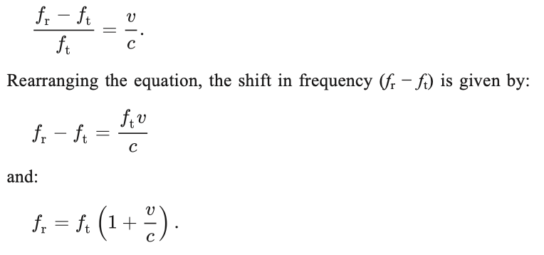
Fractional change in frequency: Relative speed divided by the speed of light.
Equations
Where:
is the transmitter frequency.
is the frequency of the received signal.
is the speed of the receiver relative to the transmitter (positive when moving towards, negative when moving apart).
is the speed of light.
Example: Car moving at 70 mph (31.29 m/s) towards a base station transmitting at 1850 MHz.
Doppler shift when car is moving away: Negative.
Doppler shift when car is moving towards: Positive.
No Doppler shift when car is directly under the base station antennas.
Importance of Doppler shift:
Large shift can move a transmission from one channel frequency to another.
OFDM uses narrow-band subcarriers, Doppler shift limits their spacing.
Frequency reuse
Restricted range of propagation is a benefit for frequency reuse.
Mobile phone networks have base stations communicating with mobile devices within cells.
Base station transmitting power serves devices up to 1 km away with adequate signal.
Inverse fourth-power law reduces interference from similar transmitters 5 km away compared to free-space propagation.
GSM (2G) uses different frequencies for transmissions in different cells.
3G and beyond have different approaches to keeping transmissions separate.
5G supports a broader range of devices and applications, in part because of its increased flexibility in how radio spectrum is allocated.
Directional antennas are used in mobile communications, with the area covered by a base station divided into sectors.
Each sector is covered by a directional antenna.
3G masts have three antennas, each covering a 120° sector.
Multiple antennas and MIMO
Performance can be improved by using multiple antennas at the transmitter, receiver, or both.
Arrays of antennas increase gain and achieve desired directional properties.
Implementation is possible with digital processing power.
Differences in signals received by two antennas placed a short distance apart are expected due to fading.
Selecting the best signal or combining received signals can improve performance.
Beam steering/beamforming uses multiple transmitter antennas to improve reception at a target device.
Relative amplitudes and phases of signals are adjusted for constructive interference at the receiver.
MIMO (multiple input multiple output) uses multiple antennas at both the transmitter and receiver.
Provides diversity with multiple paths between transmitter and receiver.
Frequency diversity: Spread spectrum and OFDM.
Spatial diversity: Multiple paths with different fading characteristics.
MIMO can provide spatial multiplexing, sending more than one stream of data at the same time.
Each receiver antenna receives a different combination of transmitted signals due to variations in fading.
Characteristics of paths are estimated and updated.
Data streams are reconstructed from received signals.
Multi-user MIMO (MU-MIMO) covers multiple users at different locations.
Same frequency is used for all users, kept separate through spatial multiplexing techniques.
Examples of MIMO:
LTE (4G) for mobile telephony.
IEEE 802.11ac and 802.11n (WiFi) for wireless networking.
Design of communication systems depends on theoretical ideas.
Noise and signal power
Transmission success is affected by noise.
Power calculation
Modulated signals have a continuous spectrum.
Noise and interference also have continuous spectra, though some have well-defined frequencies.
Total power can be measured in watts.
When power is spread over a continuous spectrum, power density is used to describe power distribution.
Power density:
Total power in a signal with a rectangular distribution is obtained by multiplying the power density by the bandwidth.
Similar considerations apply to noise.
Signal-to-noise ratio
Signal-to-noise ratio (S/N or SNR) is the signal power divided by the noise power.
The higher the S/N ratio, the less the signal is affected by noise.
Can be expressed as a simple ratio or in decibels.
Derived from signal and noise power densities.
Signal power is calculated by multiplying the signal power density by the bandwidth, and likewise with noise power.
Choosing the right receiver:
Spectrum of transmitted signal does not change, but the spectrum of the received signal through the passband does change.
Receiver B is the best option, as it capture all signal frequency components and minimise noise.
Receiver A could lose data, and receiver C would allow through more noise than necessary.
Comparing S/N ratios
To compare two S/N ratios, e.g., to see improvement by moving nearer a transmitter, noise is important.
If the noise power is the same in both places, it cancels out.
The ratio of the two signal powers is numerically the same as the ratio of the two values of S/N.
Example: Inverse square law, halving the distance increases both the signal power and the S/N ratio by four times, or 6 dB.
The ratio of the two signal powers is numerically the same as the ratio of the two values of S/N.
The effect of noise on data and error rates
Noise can cause symbols to be misinterpreted.
Factors affecting the likelihood of errors:
Increasing signal power: Reduces errors.
Increasing noise power: Increases errors.
Larger symbol set: Increases errors.
Longer symbols: May reduce errors.
Error correction can reduce the incidence of errors.
Limits to signal power, and it is not easy to reduce noise power.
Modulation techniques with many symbols increase data rate, but this advantage would be lost by using fewer symbols.
Longer symbols or repeated symbols would also reduce the data rate.
Greater bandwidth means more information can be sent.
Section 5 looks at the theoretical limitations that noise imposes on the data rate.
Section 6 considers quantifying the effect of noise on various modulation schemes.
Noise and data rate
Investigates the limits on the data rate set by varying amounts of noise.
Looks at theoretical constraints to data rate in a noise-free environment.
The sampling theorem
The first stage of analogue-to-digital conversion is to sample the signal at regular intervals.
The sampling theorem is a fundamental result in communications theory.
It puts a lower limit on the rate at which samples must be taken if a signal is to be accurately reconstructed.
Assume that the spectrum of the signal to be sampled has frequency components ranging from zero to f Hz; above f, there are no frequency components and the spectrum is zero.
The sampling theorem states that the signal can be exactly reconstructed from its samples (at least in principle) if the samples are taken at a rate exceeding 2f samples per second.
The sampling theorem is also known as the Nyquist theorem (named after Harry Nyquist).
According to the Nyquist theorem, two samples per cycle are all that is required to adequately represent an analogue signal digitally.
The Nyquist theorem states that the sampling frequency must be at least twice the highest frequency present in the signal.
Information about the signal will be lost as a phenomenon, known as aliasing, will occur when the sampling frequency is less than twice the maximum analogue signal frequency.
The necessity of the 2f limit is readily demonstrated by a counter-example.
Aliasing is an effect of the sampling rate is too low.
Data rate in a noise-free channel
The sampling theorem, or variants of it, was formulated independently by a number of people, notably Kotelnikov and Shannon.
The figure of twice the bandwidth is often referred to as the 'Nyquist rate' after Harry Nyquist (1889-1976).
More generally, what is the maximum data rate for digital data through a band-limited channel?
By band-limited, I mean that the channel only passes frequencies up to a certain value and rejects all higher frequencies.
It makes sense to send signals that are entirely or largely within the frequency range of the channel, as higher-frequency components will be lost anyway, and just represent wasted energy.
This condition can be met quite well by the digital modulation schemes that you saw in Part 2 of this block, such as QPSK and QAM.
Telegraphy in Nyquist's time used binary schemes in which each bit was represented by either a pulse or no pulse, and schemes with three different symbols (positive pulse, negative pulse or no pulse).
He also considered schemes with larger sets of symbols; modern examples would be 16-QAM or 64-QAM, with 16 or 64 different possible symbols.
His key result can be stated as follows:
The maximum rate at which symbols can be sent through a noise-free channel is 2B symbols per second (where B is the bandwidth of the channel in Hz).
To find the data rate in bits per second, the symbol rate is multiplied by the number of bits that can be represented by a single symbol.
The general formula for the number of bits per symbol, n, given by a set of M different symbols is:
.Putting these results together, the maximum data rate, D, in bits per second in a noise-free channel with bandwidth B and a set of M symbols is given by:
.
Data rate in a noisy channel
It may appear from Nyquist's formula that the data rate could be increased indefinitely just by increasing the number of different symbols in the set.
Remember, though, that this is for a noise-free channel.
As the number of symbols increases, the more difficult they are to distinguish, and the more susceptible they become to corruption by noise.
Shannon's equation
You have seen that although noise may cause errors to occur, the incidence of errors can be reduced in various ways: by using error-correcting coding, or reducing the data rate, or increasing the signal power.
Errors can generally be reduced to arbitrarily low levels, provided the data rate is low enough.
Just how low the data rate needs to be is given by a result discovered by Claude Shannon (1916-2001), a cryptographer and electronics engineer who made important contributions to the field of information theory.
He showed that there is a theoretical maximum rate at which data can be transmitted in a noisy communications channel at an arbitrarily low error rate (Shannon, 1949).
This important result is expressed mathematically as:
Where:
C is the theoretical maximum channel capacity, measured in bits per second
W is the bandwidth of the channel, in hertz
S is the signal power and N is the noise power, so that S/N is the signal-to-noise ratio
\log_2 means a logarithm to base 2 and not to the usual base 10.
Note that S/N is a simple ratio here.
Shannon's equation shows that the maximum channel capacity increases with bandwidth, as expected, and also that it increases with increasing signal-to- noise ratio.
Notice that Shannon's equation involves only these three quantities: channel capacity, bandwidth and signal-to-noise ratio.
What it does provide is a theoretical upper bound to the data rate that can be obtained with a given bandwidth and signal-to-noise ratio, known as the Shannon limit.
Limitations of Shannon's equation
Although Shannon's equation is regarded as a fundamental result in communications theory, you should be aware of its limitations.
These stem from the fact that the equation applies strictly to one particular type of noise, known as additive white Gaussian noise (AWGN).
'White noise' is not concentrated at any particular frequency, but is equally spread all over the spectrum.
'Additive' in this case means that different noise sources add together.
The term 'Gaussian' relates to the statistical distribution of the noise, which follows a bell curve.
Noise and bit error rate (BER)
A parameter of great significance, therefore, is the bit error rate (BER).
At the most basic level, this means that noise and interference can cause a demodulated received bit to differ from the original transmitted bit.
The bit error rate is the number of bits received in error divided by the number of bits transmitted in total.
Example:
The sequence of 10 bits is transmitted: 1 1 0 1 0 1 1 0 1 0 and,
After demodulation at the receiver, the sequence is recovered: 1 1 0 0 0 1 1 0 1 1.
There are two errors. The BER is therefore 2/10 = 0.2.
Plotting BER
Bit error rates are usually plotted on a graph against Eb/N0, which is an important ratio in digital communications.
Is the signal-to-noise (S/N) ratio, but more accurately Eb/N0 is the S/N ratio per bit.
The Eb term is the energy per bit:
W \cdot s \text{or joules}(J).
The N0 term is the noise power spectral density, which means it is the noise power in 1 Hz bandwidth and is given by the noise power divided by the bandwidth
W/Hz.
Because the two terms Eb and N0 have the same units, Eb/N0 is dimensionless and is usually expressed in decibels.
BER under different channel conditions
BER curves assume just AWGN is present.
However, most radio communications signals experience other effects detrimental to performance, such as multipath and fading.
BERs are much higher in these types of channel.
When channel conditions are very harsh, the BER levels off and stops reducing even at higher signal-to-noise ratios.
This is known as an irreducible BER.
These techniques can bring the curve back down towards the performance illustrated for AWGN, although this is a theoretical performance and not achievable in real radio channels.
Spectrum management
Users of the spectrum include not only broadcasters, mobile phone networks and the like, but also services unrelated to communications: radar and radionavigation, meteorological and Earth exploration satellites, and radio astronomy, for example.
Policy on issuing licences has evolved over time in the UK.
Traditionally, it was done by 'command and control', where prospective users would make proposals to operate transmitters, and licences would be issued on the merits of each case.
More recently, market mechanisms have come to the fore, with auctions for spectrum for 3G and 4G networks.
Spectrum access rights can also be traded in many cases.
Spectrum auctions have raised significant revenue, and putting a price on spectrum discourages wastage.
However, not everything is left to the market.
International and UK frameworks
Radio spectrum is managed at world level by the International Telecommunications Union (ITU).
The ITU has developed a global international treaty, the Radio Regulations, which sets out in general terms how each part of the spectrum is to be used. Frequency allocations in the Radio Regulations are either global or apply specifically to one or two of three regions of the world: the Americas, Asia Pacific, and the Europe and Africa region (which includes Russia and others).
In the UK, non-military use of the radio spectrum is licensed by Ofcom.
These are also bodies at regional level that play a role in harmonising national policies, one benefit being that products developed in one country will be directly marketable to other countries in the region. In Europe, this is done by the Electronic Communications Committee (ECC) of the European Conference of Postal and Telecommunications Administrations (CEPT).
The permitted use of radio spectrum in the UK is set out in a large document, the UK Frequency Allocation Table (UK FAT), which is periodically updated.
Alternate pages of the FAT list the allocations for the three world regions as set out by the ITU, and the corresponding national allocations for the same frequencies.
The Radio Regulations recognise two classes of user, primary and secondary: