Quantifying Uncertainty
Acting Rationally
Rational agents with perfect knowledge of the environment*
‣ can find an optimal solution by exploring the complete environment;
‣ can find a good (but perhaps suboptimal) solution by exploring part of the environment using heuristics.
*: rarely the entire environment
Acting Rationally under Uncertanty
What should rational agents do if they don’t have perfect information? (Poker)
‣ Maximize performance by keeping track of the relative importance of different outcomes and the likelihood that these outcomes will be achieved.
Dealing with Uncertanty
Logic is insufficient
‣ toothache ⇒ cavity ?
‣ toothache ⇒ cavity ∨ gum problem
‣ toothache ⇒ cavity ∨ gum problem ∨ abscess
‣ toothache ⇒ cavity ∨ gum problem ∨ abscess ∨ sinus block ∨ …
‣ cavity ⇒toothache ?
Only an exhaustive list of possibilities on the right hand side will make the rule true.
Logic is insufficient
‣ Laziness: it’s too much work to make and use the rules.
‣ Theoretical Ignorance: we don’t know everything there is to know.
‣ Practical Ignorance: we don’t have access to all of the information.
→ Replace certainty (logic) with degrees of belief (probability)
Probability Theory
‣ Probability statements are usually made with regard to a knowledge state.
‣ Actual state: patient has a cavity or patient does not have a cavity
‣ Knowledge state: probability that the patient has a cavity if we haven’t observed her yet.
Decision Theory
Decision theory = probability theory + utility theory
Principle of maximum expected utility (MEU)
‣ An agent is rational if and only if it chooses the action that yields the highest expected utility. Expected = average of outcome utilities, weighted by probability of the outcome
Acting under Uncertanity
What if: You have to choose between a 0.8 chance of getting 4000 EUR, and a 100 % chance of getting 3000 EUR ( and a weel, utility, probabilty, expected utility)
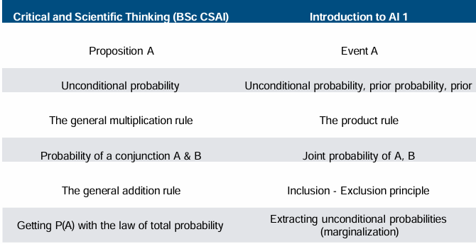
Probability Terminology Map
Possible Worlds
‣ The term possible worlds originates in philosophy the actual world could have been different. in reference to ways in which
‣ In statistics and AI, we use it to refer to the possible states of whatever we are trying to represent, for example, the possible configurations of a chess board or the possible outcomes of throwing a die.
‣ The term world is limited to the problem we aretrying to represent.
‣ A possible world (ω(lowercase omega)) is a state that the world could be in. capital omega
‣ The set of possible worlds ( Ω(capital omega) ) includes all the states that the world could be in. In other words, Ω must be exhaustive.
‣ Each possible world must be different from all the other possible worlds. In other words, possible worlds must be mutually exclusive.
Sample space
Ex. Throwing dice
Sample space = Set of all possible worlds: Ω
‣ Ω = {(1,1), (1,2), … (6,5), (6,6)}
Possible world = element of the sample space: ω
‣ w ‣ ω₁ = (1,1)
‣ ω₃₆ = (6,6)
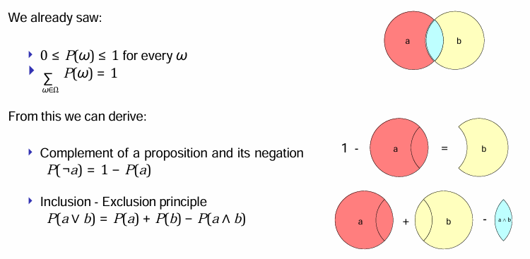
0 ≤ P(ω) ≤ 1 for every ω and∑ P(ω) = 1
Random variables and Events
Random variable
‣ Function that maps from a set of possible worlds to a domain or range.
‣ Typically written with upper case letter
Event
‣ Set of worlds in which a proposition holds
‣ Probability of an event: sum of probabilities of the worlds in which a proposition holds Example
‣ Random variable: Total with range {2, …, 12}
‣ Proposition "rolling 11 with two dice": P(Total = 11)
‣ Event: set of worlds in which the proposition holds: {(5,6),(6,5)}
‣ Probability of event: P((5,6)) + P((6,5)) = 1/36 + 1/36 = 1/18
(Un)conditional Probabilities
Unconditional probabilities: Degree of belief in propositions in the absence of other information.
‣ Also known as prior probabilities or priors.
Conditional probabilities: Degree of belief given other information.
‣ Example: rolling a double if the first dice is 5
‣ P (doubles ∣ Dice1 = 5
Conditional Probabilities
Computing conditional probabilities
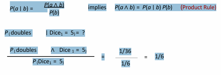
Joint probability distribution:
‣ P(Toothache, Cavity) = P(Toothache ∣ Cavity)P(Cavity)
‣ Boldface P means “for all possible values of the random variable”.
‣ A probability model is completely determined by the full joint probability distribution (the joint distribution for all of the random variables).
‣ E.g., P(Cavity, Toothache, Catch) = 2x2x2 table
Probability Axioms
Probabilistic Inference
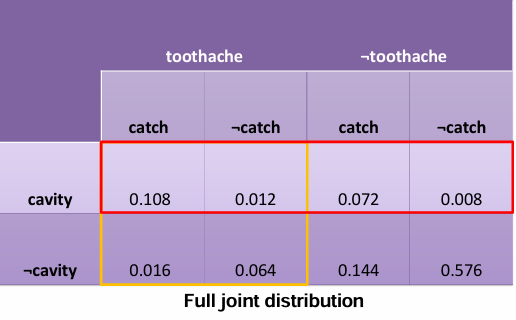
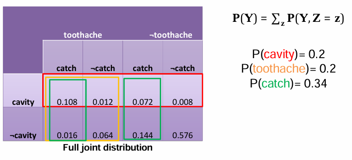
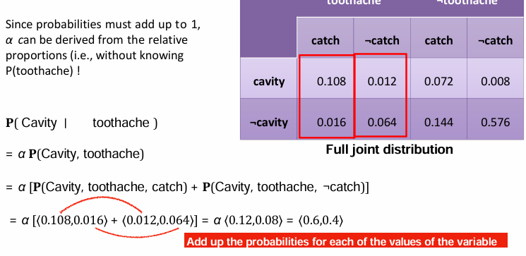
P(cavity ∨toothache)= 0.108 + 0.012 + 0.072 + 0.008 + 0.016 + 0.064 = 0.28
Extracting unconditional probabilities(marginalization)
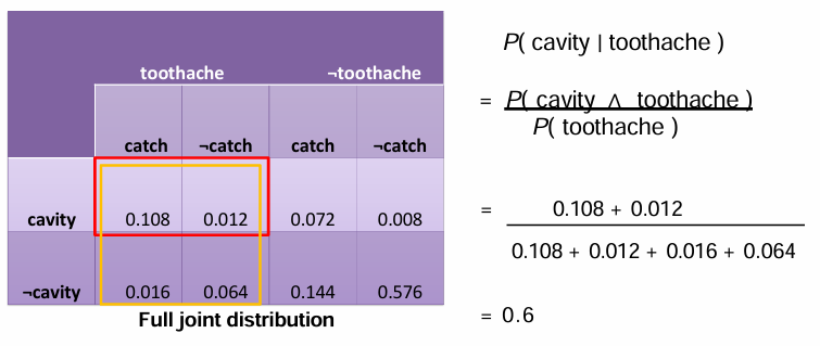
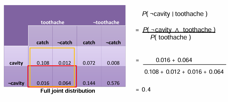
Computing conditional probabilities
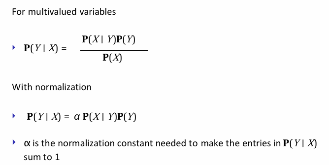
Normalization constant
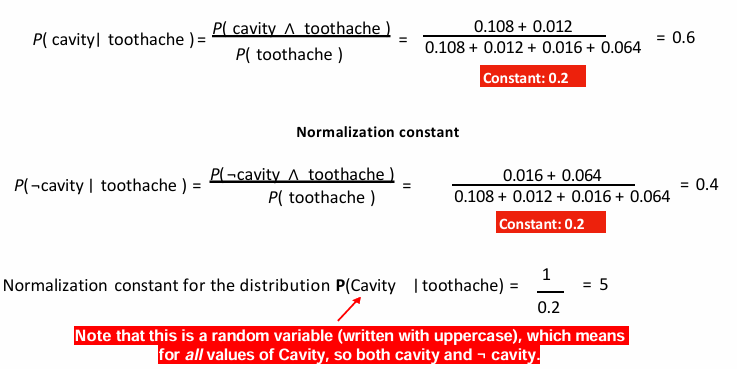
Normalization
A general inference procedure
General form of the procedure described in previous slide:
P(X ∣ e) = α P(X,e) = α∑ P(X,e,y)
→ Can answer questions about the probability distribution of a discrete random variable X, given evidence variables E, and unobserved variables Y.
Does not scale well. For n variables with two values each:
‣ space complexity = O(2n)
‣ time complexity = O(2n)
‣ (i.e., complexity doubles with every additional variable)
Adding extra variables
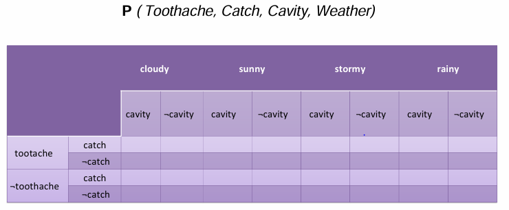
Full joint distribution with 32 elements…
Independence
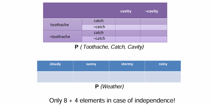
‣ Assumptions about independence are usually based on domain knowledge.
‣ Independence drastically reduces the amount of information needed to specify the full joint distribution
For instance: rolling 5 dice
‣ Full joint distribution: 65 = 7776
‣ Five single variable distributions: 6 * 5 = 30
Conditional Independence
Example:
‣ Catch and toothache are not independent: if the probe catches, then it is likely that the tooth has a cavity and that this cavity causes a toothache.
‣ However, toothache and catch are independent, given the presence or absence of a cavity.
• If a cavity is present, then whether there is a toothache is not dependent on whether the probe catches, and vice versa.
• If a cavity is not present, then whether there is a toothache is not dependent on whether the probe catches, and vice versa.
→ P(toothache, catch | cavity) = P(toothache | cavity)P(catch | cavity)
P(X,Y|Z) = P(X|Z) P(Y|Z)
Bayes’ Rule- Derivation
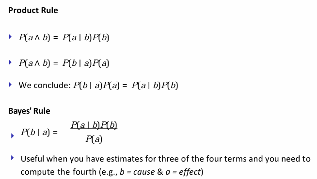
Bayes’ Rule
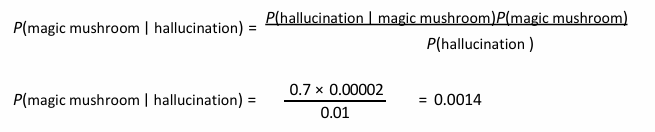
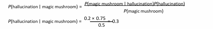
Bayes’ Rule - Diagnostic application
Determining the probability of a cause given a certain effect (diagnosis).
‣ Example: what is the probability that you ate a magic mushroom if you are hallucinating?
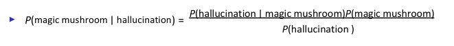
A patient comes into the hospital with hallucinations after lunch.
‣ Magic mushrooms cause hallucinations 70% of the time.
‣ The prior probability that someone ate magic mushrooms for lunch is 1/50,000.
‣ The prior probability that someone who comes into the hospital has hallucinations is 1%.
Bayes’ Rule- Causal application
Determining the probability of an effect given a certain cause (medication).
‣ Example: what is the probability that you will hallucinate when eat a magic mushroom?
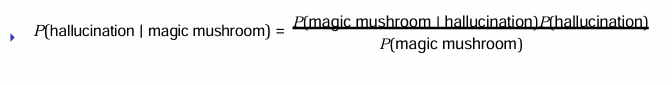
A devoted researcher does experiments with psychoactive substances once a month. Over the course of the last year, the researcher did 12 experiments
‣ the researcher hallucinated 9 times out of 12.
‣ out of the 10 times the researcher was hallucinating, two were attributable to magic mushroom use.
‣ half of the experiments involved magic mushrooms.
Scaling up inference?
Neither inferring from the full joint distribution, nor a straightforward application of Bayes’ rule scale up well
‣ Conditional independence assertions can decompose full joint distribution into smaller pieces.
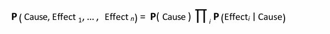
‣ If we assume that a single cause influences a number of independent effects → Naive Bayes model
Summary
‣ Logic is insufficient to act rationally under uncertainty.
‣ Decision theory states that under uncertainty, the best action is the one that maximizes the expected utility of the outcomes.
‣ Probability theory formalizes the notions we require to infer the expected utility of actions under uncertainty.
‣ Given a full joint probability distribution, we can formalize a general inference procedure.
‣ Bayes’ rule allows for inferences about unknown probabilities from conditional probabilities. ‣ Neither the general inference procedure, nor Bayes’ rule scale up well.
‣ Assuming conditional independence allows for the full joint probability distribution to be factored into smaller conditional distributions → Naive Bayes.