week 7/8 - factorial anova
FOR EXPERIMENTAL QUASO EXPERIMENTAL DESIGN. BETWEEN SUBJECTS DESIGN (ALL IV groups)
One-way anova - oneway DV IV
effect size = sum square between/ sum square total
effect size in pairwise comp
cohen’s D - ?
Factorial Anova
one DV numerical DV
IV - multiple, two or levels for each IV
They are all fully crossed
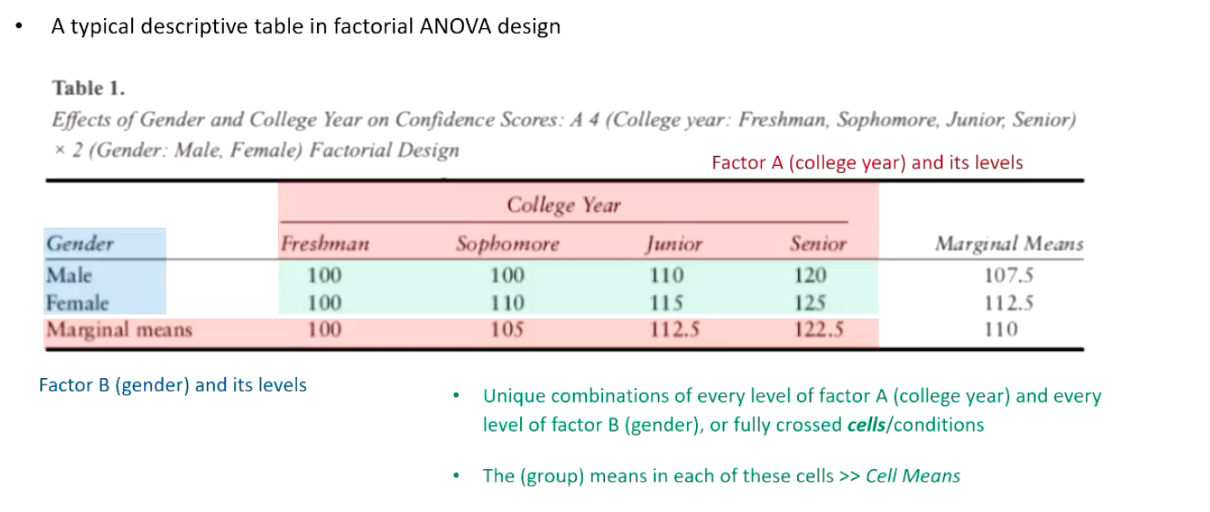
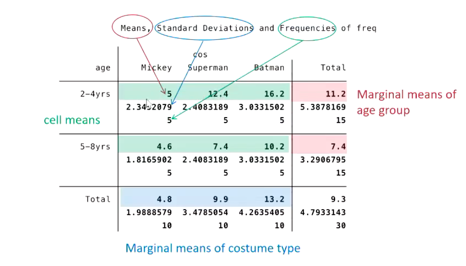
costume type & age
mickey, superman, batman
2-4 years, 5-8 years
why do we factorial instead of multiple one way anovas - moderating effects - one IV may change the direction of the other IV on the DV
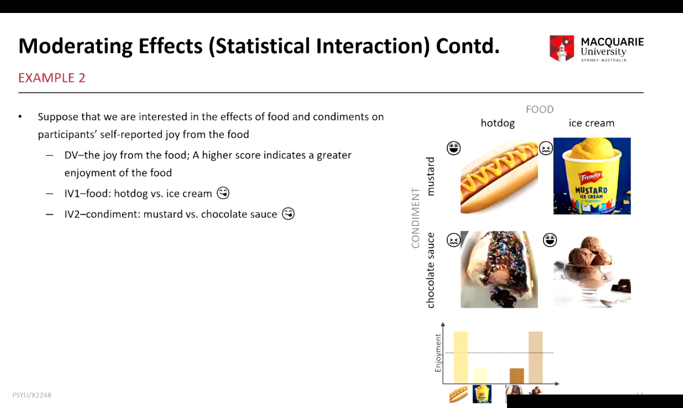
presence of the 2nd IV changed the enjoyment of food DV - type of condiments put on the food changes the direction of how much we enjoy the food
F anova terminology
IVs are called factors
Groups are called levels
Which group means are compared
Statistical Analysis
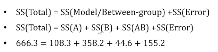
Factorial ANOVA variance partitioning
within-group: variance is still represented by the variation within each group
between-group: variances can be divided into three parts
between group variances under factor A
between group variances under factor B
the moderating effect (interaction) between A and B
Total sum of squares - total variability in the DV (deviations of all observations from the gran mean) is represented by total some of squares
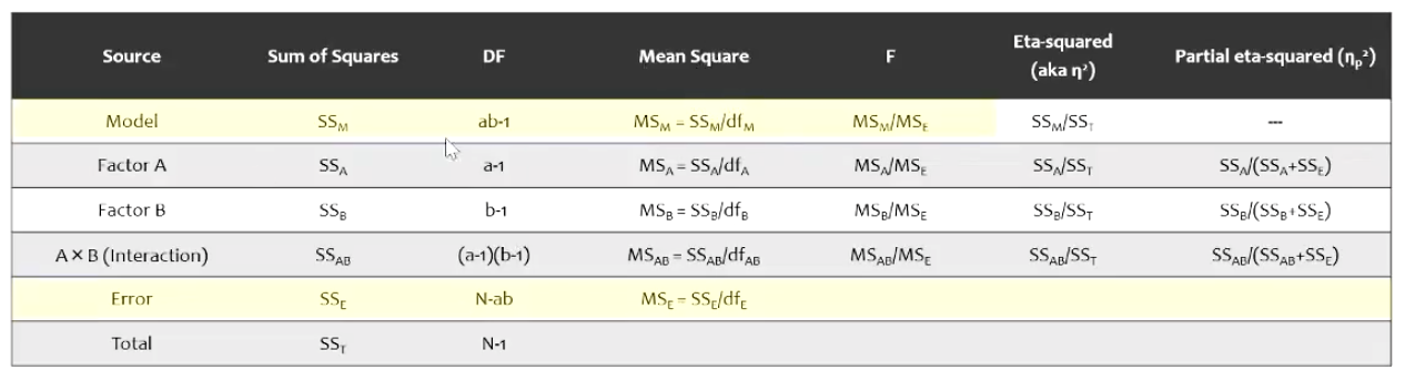
summary table
Assumptions for FACTORIAL ANOVA
numeric DV: DV is measured on an interval/ ratio scale
independence of observations: no relationship between observations within or between each combined levels of IV
random allocation of subjects to groups
Normality: DV is normally distributed for each combined levels of IVs
Homogeneity/ homoscedasticity: equal variance for each combined levels of IVs
cohend’s D

IN STATA
label bivariate data to summarise statistics; egen (new name) = group (IV IV), label
tabstat freq, by(new name) stat(n mean sd skewness kurtosis)
tab IV1 IV2, summarize (DV) - marginal cell and mean table
line graphs; anova freq IV1##IV2 - margins IV1#IV2 and then we do the marginsplot
bar plot: cibar freq, over (IV2 IV1)
NORMALITY: visualisation of a histogram OR shapiro wilk
histogram freq by (IV1 IV2) / by IV1 IV2 sort: swilk freq
normality is violated if pvalue is less than 0.05 - it needs to be greater than 0.05 to do second analysis
HOMOGENEITY: Levenes test
robvar freq, by (new_name)
p value needs to be larger than 0.05
Fit appropriate stat model (s)
Omnibus F-test (main effect+interaction)
ANOVA: anova DV IV1 IV2 IV1#IV2
anova DV IV1##IV2
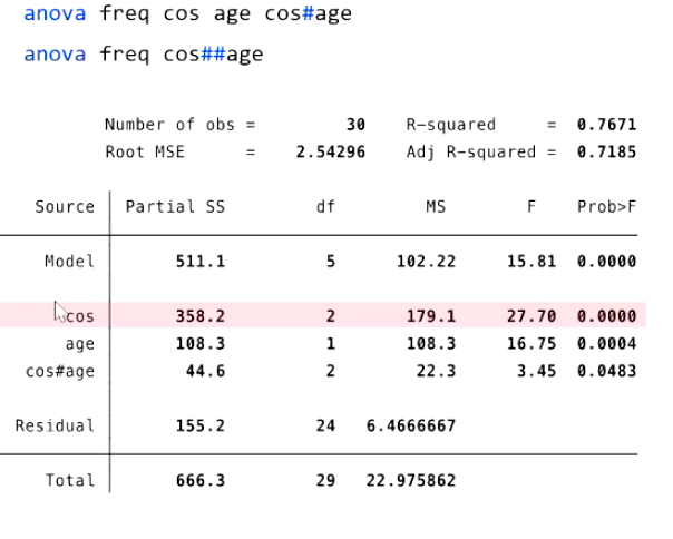
if the p value is less than 0.05 - we can reject the null hypothesis
only need to do a follow up for factors more than 3 so we see where the difference is but not for 2 levels as we can say one group is significantly diff than the other
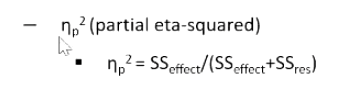
effect size; estat esize
F - value is calculated by MSeffect/MSresidual
Conclusion
main effects: what is the effect of a factor across all levels of another factor(s) How do the means differ ignoring all other factors
interaction effects: is the effect of one factor the same or different at various levels of another factor(s)Are there different at each level
FA - compares group means through between vs within group variances but between group variances can be further parted into variances
follow-up analysis - simple effect analysis
Calculations
cohens’d

F value
effect size