Constraint Satisfaction Problems
Assumptions about the world:
a single agent
deterministic actions
fully observed state
discrete state space
Identification: assignments to variables
the goal itself is important, not the path
all paths are at the same depth
CSPs are a specialized class of identification problems
Standard Search Problems:
state is a “black box”: arbitrary data structure
goal test can be any function over states
successor function can also be anything
Constraint Satisfaction Problems (CSPs):
A special subset of search problems
state is defined by variables X, with values from domain D
goal test is a set of constraints specifying allowable combinations of values for subsets of variables
Ex. Map of Australia
variables: different regions: WA, NT, Q, NSW, V, SA, T
domains: D = {red, green, blue}
constraints: adjacent regions must have different colours
Implicit: WA ≠ NT
Explicit: (WA, NT) ∈ {(red, green), (red, blue), …}
solutions are assignments satisfying all constraints
ex. {WA = red, NT = green, Q = red, NSW = green, V = red, SA = blue, T = green}
there are many solutions
Constraint Graph:
binary CSP:
each constraint relates two variables
binary constraint graph:
nodes are variables, arcs show constraints
general-purpose CSP algorithms use the graph structure to speed up search
Varieties of CSPs:
Discrete Variables
finite domains
size d means O(dt) complete assignments
infinite domains (integers, strings, etc)
linear constraints solvable, nonlinear undecidable
Continuous Variables
linear constraints solvable in polynomial time by LP methods
Varieties of Constraints
unary constraints involve a single variable (equivalent to reducing domains)
binary constraints involve pairs of variables
higher-order constraints involve 3 or more variables
Standard Search Formulation:
states defined by the values assigned so far (partial assignments)
initial state: the empty assignment, {}
successor function: assign value to an unassigned variable
goal test: the current assignment is complete and satisfies all constraints
Remember Australia colour problem:
BFS would take forever because all the solutions are at the bottom
DFS would also take a long time
Backtracking Search!
Backtracking Search:
one variable at a time
check constraints as you go
“incremental goal test”
improving this:
ordering: which variable should be assigned next?
filtering: can we detect failure earlier?
structure: can we exploit the problem structure?
Filtering:
keep track of domains for unassigned variables and cross off bad options
forward-checking:
cross off values that violate a constraint when added to the existing assignment
doesn’t recognize failure until there are no options
Consistency of a Single Arc:
An arc X → Y is consistent iff for every x in the tail there is some y in the head which could be assigned without violating a constraint
“delete from the tail”
forward checking: enforcing consistency of arc pointing to each new assignment
Arc Consistency of an Entire CSP:
a simple form of propagation makes sure all arcs are consistent
Important: if X loses a value, neighbours of X need to be rechecked
arc consistency detects failure earlier than forward checking
What’s the downside?
runtime: O(n2d3)
Limitations of Arc Consistency:
can have one, multiple, or no solutions left after
Ordering:
Variable Ordering:
minimum remaining values (MRV)
choose the variable with the fewest legal left values in its domain
why min instead of max?
“fail fast” because you have to assign every variable anyways
“most constrained variable”
Value Ordering:
given a choice of variable, choose the least constraining value (LCV)
rules out the fewest remaining values
Combining these ordering ideas makes many things possible!
K-Consistency:
increasing degrees of consistency
1-consistency (node consistency): each single node’s domain has a value which meets that node’s unary constraints
2-consistency (arc consistency): fior each pair of nodes, any consistent assignment to one can be extended to the other
K-consistency: for each k nodes, any consistent assignment to k-1 can be extended to the kth node
higher k more expensive to compute
strong k-consistency: also k-1, k-2, … 1 consistent
means we can solve without backtracking
Structure:
Extreme case: independent subproblems
identifiable as connected components of the constraint graph
break up a graph into subproblems of only c variables
not useful
Tree-Structured CSPs:
Theorem: if the constraint graph has no loops, the CSP can be solved in O(n d2) time
this property also applies to probabilistic reasoning
Algorithm:
order: choose a root variable, order variables so that parents precede children
remove backward: for i = n : 2, apply RemoveInconsistent(Parent(Xi), Xi)
assign forward: for i = 1 : n, assign Xi, consistency with Parent(Xi)
Runtime = O(n d2)
Nearly Tree-Structured CSPs:
conditioning: instantiate a variable, prune its neighbours’ domains
cutset conditioning: instantiate (in all ways) a set of variables such that the remaining constraint graph is a tree
cutset size c gives runtime O((dc) (n - c) d2)
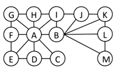
ex. which is the smallest cutset on the below tree?
Tree Decomposition:
Idea: create a tree-structured graph of mega-variables
each mega-variable encodes part of the original CSP
subproblems overlap to ensure consistent solutions
Iterative Improvement:
local search methods typically work with “complete” states, ie. all variables assigned
to apply to CSPs:
take an assignment with unsatisfied constraints
operators reassign variable values
no fringe
algorithm:
variable selection: randomly select any conflicted variable
value selection: min-conflicts heuristic:
choose a value that violates the fewest constraints
performance of min-conflicts:
R = number of constraints / number of variables
Summary of CSPs:
CSPs are a special kind of search problem
states are partial assignments
goal test defined by constraints
Basic solution: backtracking search
speed-ups:
ordering
filtering
structure
Iterative min-conflicts is often effective in practice
Local Search:
tree search keeps unexplored alternatives on the fringe (ensures completeness)
local search: improve a single option until you can’t make it better
new successor function: local changes
generally much faster and more memory efficient
but incomplete and suboptimal
Hill Climbing:
simple, general idea
start wherever
repeat: move to best neighbouring state
if no neighbours better than current, quit
not complete or optimal
Simulated Annealing: escape local maxima by allowing downhill moves
theoretical guarantee: if T decreases slowly enough, will converge to optimal state
Genetic Algorithms: uses a natural selection metaphor
keep best N hypotheses at each step based on a fitness function