AP Econ A & O

Group A: 2.3, 2.7, 3.2, 3.7, 4.7

Group O: 3.5, 3.8, 4.6, 6.5, 6.6

Group A:

(Topic 2.3: Unemployment)

• Population: total # of people in a country

• Working Age Population: # of people ages 16+

• Civilian Labor Force: # of people classified as either employed or unemployed (military & institutionalized are excluded)

• Employed: people who have worked at least 1 hour in the last 2 weeks (includes part-time and full-time employment)

• Unemployed: people not classified as employed but available for work and have submitted a job application in the last 4 weeks

• Marginally Attached Worker: people available for work within the last 12 months not classified as employed or unemployed

• Discouraged Worker: people previously classified as unemployed who exited the civilian labor force without finding employment

• Calculating Unemployment: Labor Force Participation Rate: (Civilian Labor Force/ Working Age Population) * 100

• Actual Unemployment Rate: (Number of people classified as unemployed/ civilian labor force) * 100

Types of unemployment:

• Frictional Unemployment is associated with voluntary job search and entry into the civilian labor force

• Structural Unemployment is associated with either a skill or geographic mismatch between individuals and available jobs. Can also be seasonal unemployment

• Cyclical Unemployment is associated with joblessness caused by economic recession

Natural Rate of Unemployment (NRU)

• Natural Rate of Unemployment (NRU): Frictional rate of unemployment + Structural rate of unemployment (just think of cyclical not being included)

• NRU occurs at full employment output. This means that employment resources are used efficiently (think PPC)

• Cyclical Unemployment can be calculated by Actual Unemployment Rate - NRU

(Topic 2.7: Business Cycles)

• Output: can refer to Real or Nominal GDP, Real or Nominal GDP per capita, or growth rate

• Time can be measured in quarters (3-month time periods) or years

• Potential growth (output economy can produce at constant inflation) vs actual growth (growth that has actually happened in real life) (2 separate curves)

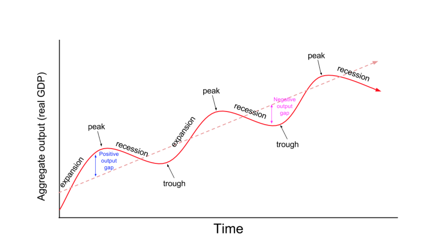
Phases in the business cycle describe what is happening to our economy

• Expansion: output is increasing, and employment is rising

• Recession: output is decreasing, and employment is falling

Turning points are found where increasing goes to decreasing and vice versa. These are referred to as peaks and troughs.

(Topic 3.2: Multipliers)

• Autonomous expenditure: (independent spending) spending by C (households), I (firms), or G (government) on any extra non-necessity goods and services

• If autonomous spending by C, I, or G changes by $1, the AD will change by greater than $1

Definitions:

• Disposable income (Yd): Gross income - income tax

• When you earn income, you can either spend (consume) or save that money

• APC: Average propensity to consume is your likelihood of spending your income. The formula is: Consumption Amount/ Disposable Income

• APS: Average propensity to save is your likelihood of saving your income. Formula is savings amount/ Disposable Income

• Margin: Additional

• Equilibrium income: one person’s spending is another person’s income

Formulas:

• MPC: The percentage of an additional $1 earned in Yd spent on consumption.

  • The formula is change in consumption/ change in Yd

• MPS: The percentage of an additional $1 earned in Yd that is saved.

  • The formula is Change in Savings/ Change in Yd

• Tax multiplier quantifies the total change in AD that results from an initial change in taxes or transfer payments.

  • The formula is -(MPC/1-MPC) or

    -(MPC/MPS)

    • There is a negative sign because when taxes increase, aggregate demand decreases

• Transfer multiplier: (MPC/1-MPC) or (MPC/MPS)

• Spending multiplier: (1/MPS) or 1/(1-MPC)

• Spending is going to multiply across the economy and have a large impact on GDP

  • Initial Change x Spending Multiplier

Applying these multipliers/ formulas:

• Change in taxes: Total change in AD = initial change in taxes x tax multiplier

• Change in transfers: Total change in AD = initial change in transfers x transfer multiplier

(Topic 3.7: Long Run Self-Adjustment)

• Long-run self-adjustment: when an economy is in an inflationary or recessionary gap, the SRAS curve will automatically self-correct and shift to bring the economy back to equilibrium

• The adjustment is created through the natural results of the free market

• The shift in SRAS will be driven by both businesses and workers (in theory, but in reality, this would take a long time)

• When in a recessionary gap, businesses will lower prices and workers will be willing to accept lower wages

  • Both actions will result in a decrease in the price level (deflation) and a decrease in the Ur

• When in an inflationary gap, businesses will increase prices to bring outputs to a manageable level, and workers will demand higher wages for increased production

  • Both actions will lead to an increase in price level (inflation) and an increase in the Ur

(Topic 4.7: Loanable Funds Market)

• Loanable Funds Market: represents how much money in the form of a loan that consumers, businesses, and governments are requiring

  • determined by the expectation of return on investment

How much consumers pay for borrowing money:

• Uses the RIR instead of the NIR since loans are usually taken over a longer period of time

• RIR = NIR - Inflation

Graphing the Loanable Funds Market

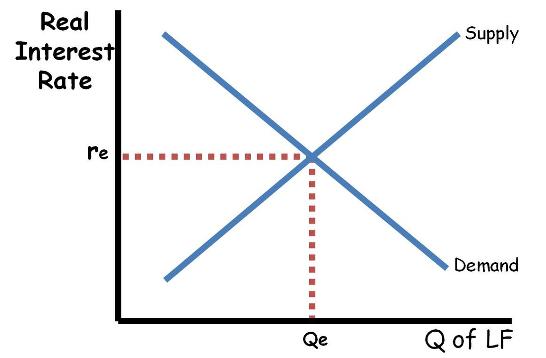Demand for loans:

• Represents the amount of loans being demanded by individuals (ex. mortgages), producers (business loans), and governments (bonds)

• Follows the same typical laws of demand. High demand at low price (RIR), low demand at high prices (RIR)

Supply of loans:

• Follows the same laws of supply. Low supply at low price (RIR), high supply at high prices (RIR)

• The supply of loans come from customer deposits

• In a “Closed Economy” (only domestic investments), supply is equal to national savings (private + public savings)

• In an “open Economy” (allows for foreign investment), supply is equal to national savings + “net capital inflow” (foreign investment)

Disequilibrium in loanable funds market:

• When RIR are too low (compared to equilibrium) there will be a shortage of loanable funds

• When RIR are too high (compared to equilibrium) there will be a surplus of loanable funds

• In both cases, biding up or down the price will result in a return to equilibrium

Determinants (shifters) of demand:

Anything that impacts the profit potential of new investments:

• Changes in economic outlook (positive = rightward shift, negative = leftward shift)

• Investment tax credits (increase = rightward shift, decrease = leftward shift)

• Corporate income taxes (increase = leftward shift, decrease = rightward shift)

• Productivity of new capital increase (increase = rightward shift, decrease = leftward shift)

• Real GDP (increase = rightward shift, decrease = leftward shift)

Group O:

(Topic 3.5: Equilibrium in the AS/ AD Model)

• Surplus is a point at which supply>demand

• Surplus is corrected by a lowering of the price level until Equilibrium is reached

• Shortage is a point at which demand>supply

• Shortage is corrected by bidding the price level up until equilibrium is reached

• Long run equilibrium is when current output is represented by a vertical LRAS curve labeled Yf

• Short run output graphs are created by changing economic conditions. These can create “recessionary gaps” and “inflationary gaps”

• A recessionary gap occurs when the current output YC< maximum potential output Yf

• Ur is > NRU

• An inflationary gap occurs when the current output Yc>maximum potential output Yf

• Ur is < NRU

  

(Topic 3.8: Fiscal Policy)

• Fiscal Policy: Policy implemented by governments to intervene when the economy is in an inflationary or recessionary gap to bring the economy back to full employment (equilibrium)

• The tools of fiscal policy are: 1. government spending 2. taxation

  • both tools impact aggregate demand, whereas the long run self-adjustment affects aggregate supply

Recessionary Gap:

• When the economy is in a recessionary gap, unemployment is growing, price level is decreasing, and productivity is decreasing

• The government will respond to this with an “expansionary fiscal policy”

• Expansionary fiscal policy will increase spending or decrease taxes or both

• Government spending has a direct impact on AD, cutting taxes has an indirect impact on AD

  • Both will shift AD to the right, but the spending will have a greater effect

Inflationary Gap:

• When the economy is in an inflationary gap, unemployment is decreasing, price level is increasing, and productivity is increasing but at an unsustainable rate

• The government will respond to this with a “contractionary fiscal policy”

• Contractionary fiscal policy will decrease spending or increase taxes or both

• Government spending has an indirect impact on AD, increasing taxes has an indirect impact on AD

• Both will shift AD to the left, but the spending will have a greater effect

(Topic 4.6: Monetary Policy)

• Monetary Policy: A central bank’s policies of influencing nominal interest rates and money supply to help achieve price stability and full employment

• The Fed: The Federal Reserve Bank is the central bank of the United States and most powerful economic institution in the world, its main responsibilities are to set interest rates, manage the money supply, and regulate financial institutions

• Interest Sensitive Spending: Spending in the form of investment (firms) and consumption (individuals)

• Reserve Requirements: amount of cash that banks must hold in reserve against deposits made by their customers

• Discount Rate: Rate at which commercial banks borrow money from each other. AKA “Federal Funds Rate” and the “Overnight Interbank Lending Rate”

Background:

• When banks are unable to meet the reserve requirement, they can:

  • Call in loans

  • Sell assets

  • Borrow from the central bank (discount rate)

  • Borrow from the other commercial banks (policy rate)

Central banks often set a target range for the policy rate to guide monetary policy though they have no legal or customary power over the interest rates banks charge.

Types of Monetary Policy:

• Expansionary Monetary Policy: When the central bank decreases nominal interest rates in the short run to help get an economy out of a recessionary gap.

  • Lower interest rates = money is less expensive to borrow = so more interest sensitive spending = increase in AD

• Contractionary Monetary Policy: When the central bank increases nominal interest rates in the short run to help get an economy out of an inflationary gap

  • Higher interest rates = money is more expensive to borrow = less interest-sensitive spending - decrease in AD

Limitations of Monetary Policy:

• Limitations of Monetary Policy are known as “lags”

  • Recognition lag & impact lag

• Recognition Lag: Can take the central banks a long time to collect and analyze the data needed to recognize problems in the economy

• Impact Lag: It can take the central banks a long time for the economy to adjust after the policy action is taken

The tools to implement change by the central bank depends on the type of reserve framework the nation is working in. Two types of reserve frameworks:

1. Limited Reserves Framework

2. Ample Reserves Framework

Limited Reserves Framework:

A banking system where:

• Commercial banks hold required reserves and possibly also some excess reserves

• Monetary policy is focused on changing the supply of excess reserves and, therefore, the money supply

Monetary policy tools:

• Required Reserve Ratio: Percentage of demand deposits banks must hold in their reserves

  • If the required reserve ratio decreases, banks have more in excess reserves to lend, so money supply increases and NIR fall

  • If the required reserve ratio increases, banks have less in excess reserves to lend, so money supply decreases and NIR rise

• Discount Rate: the interest rate commercial banks must pay to borrow from the central bank

  • If the discount rate decreases, banks are encouraged to lend more, so money supply increases and NIR fall

  • If the discount rate increases, banks are encouraged to lend less, so money supply decreases and NIR rise

• Open-Market Operations (OMO): The central bank buying and selling of government bonds (securities) from commercial banks

  • When the central bank buys bonds (OM purchases) from commercial banks, banks’ excess reserves increase (bc they’re receiving money from central banks for the bonds they sold), so money supply increases and NIR fall

  • When the central bank sells bonds (OM sale) to commercial banks, banks’ excess reserves decrease (bc they’re losing money from central banks for the bonds they purchased), so money supply decreases and NIR rise

The Effect of the Money Multiplier:

Reminder: Money multiplier is the maximum POSSIBLE value or POTENTIAL increase in the money supply

It assumes 1) banks hold no excess reserves, 2) borrowers spend their entire loans, 3) customers hold no cash

MM: 1/Required Reserve Ratio

The maximum possible change to the money supply as a result of an can be calculated as:

Change to money supply = (OMO amount)(MM)

Also:

• Open-Market Operations cause changes in reserves so the monetary base changes (M0… bank reserves and currency in circulation)

• In limited reserve environments the effect of an Open-Market Operation on the money supply is greater than the effect on the monetary base because of the money multiplier

• An increase in excess reserves (Open-Market Purchases) leads banks to make more loans, which leads to more deposits, creating more excess reserves which allows for more loans and so on

• A decrease in excess reserves (Open-Market Sales) works in the opposite way

Ample Reserves Framework:

A banking system in which:

• Reserves in central bank are abundant

• Required reserve ratio is zero

• Changing the money supply no longer linked to changes in the nominal interest rate

• Interest rate changes are brought about through changes to administered interest rates

Graphing:

A money market graph is NOT used to model a banking system with ample reserves. Instead you will draw a “Reserve Market Model Graph”

Remember: Central banks often set target ranges for their policy rate. This policy rate plays an important role in the model used for the ample reserves framework.

The policy rate is set at the intersection of Sr (Supply of reserves) and Dr (Demand for reserves)

Remember the policy rate is the overnight inter bank lending rate. In the US it is the federal funds rate.

On the graph, the Sr will always go through the lower bound of the Dr. If it was going through the sloping portion, it would represent a limited reserves framework.

Additionally, any changes in Open-Market Operations would shift the supply of reserves, but the NIR would remain unchanged.

Monetary Policy tools:

Effects on the administered interest rates:

• Interest on reserves (IOR): the interest rate commercial banks earn on the funds in their reserve balance accounts with the central bank

  • Rather than hold excess reserves, the commercial banks will put their money into the central bank to earn interest

  • Serves as the central bank’s primary monetary tool

  • Increases (or decreases) to Interest on reserves move up (or down) the lower bound on the reserve market model graph

• Discount rate: the interest rate commercial banks must pay to borrow from the central bank

  • Typically adjusted in the same manner as interest on reserves

  • Increases in the discount rate increase the upper bound on the reserved market model graph, decreases move it down

• A decrease in administered rates (IOR and discount rate) lead to a decrease in the policy rate and subsequently a decrease in other NIR.

  • This is an expansionary policy because interest sensitive spending will increase and so will aggregate demand

• A lower discount rate will encourage banks to borrow more and lend (increasing money supply) and a lower IOR will have the same effect since they profit more from lending than storing reserves in the central bank.

• The opposite is true for contractionary policy

Simplified Explanation for 4.6:

• The Central Bank can adjust interest rates and money supply to fix the economy

• In a limited reserves framework, the central bank aims to affect the amount of excess reserves the bank holds

• The more excess reserves, the more the bank can loan. The less excess reserves, the less it can loan

• The tools are reserve requirements, discount rate, and open-market purchases or sales (bonds)

• In a ample reserves framework (ARF), the central bank (CB) aims to control how much banks can loan through administrative rates

• Similar to limited reserves framework, adjusting discount rate works in a similar way

• In the ARF, banks are incentivized to keep their excess reserves in the central bank to earn interest

• The CB also controls money supply by adjusting how much interest they offer banks to hold their money

• If they offer them a high interest rate, less money is loaned out. If they offer a lower interest rate, more money is loaned out

(Topic 6.5: Changes in Foreign Exchange Markets and Net Exports)

Reminder: The shifters of AD are Consumption, Investment, Government Spending, and Net Exports

• Changes in the relative price of goods changes net exports

• Changes in currency value causes a change in the relative price of goods

When the US dollar appreciates in value, American goods become more expensive relative to the goods of other countries (USD can buy more for fewer foreign currency)

• This will cause US exports to decrease (what they’re selling)

• Additionally, this will cause US imports to increase (what they’re importing in) because foreign goods are now cheaper in comparison

• As a result Net Exports (Xn) will decrease causing AD to decrease

(Topic 6.6: Real Interest Rates and International Capital Flows)

• In an open economy (one that interacts with importing and exporting with different countries), differences in real interest rates across countries change the relative values of domestic and foreign assets

• Financial capital will flow toward the country with the relatively higher interest rates because of rate of return

  • This will affect the balance of the CFA (Capital and Financial Account) mainly due to the purchase of bonds, currency, CDs etc.

Central banks can influence the domestic interest rate in the short run which in turn will affect net capital inflow

• The effect of capital inflows and outflows are shown in the loanable funds graph model

• A capital inflow shifts supply of loanable funds (LF) to the right

• A capital outflow shifts supply of LF to the left

Causes of the shift are:

1) Monetary Policy: nominal interest rate

• Expansionary: rates decrease (as well as inflow)

• Contractionary: rates increase (as well as inflow)

2) Demand for Money

• Increase in demand: rates increase (as well as inflow)

• Decrease in demand: rates decrease (as well as inflow)

3) Government Budget Balance

• Deficit rates increase (crowding out) (as well as inflow)

• Surplus: rates decrease (as well as inflow)

4) Household saving behavior

• Increase: rates decrease (as well as inflow)

• Decrease: rates increase (as well as inflow)