Module 6: Profit Maximization in Perfectly Competitive Markets

Four Market Structure

• Perfect Competition

• Monopoly

• Monopolistic Competition

• Oligopoly

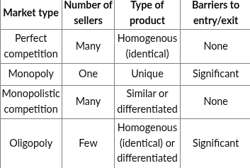
Perfect Competition

• Many sellers or producers in market/industry

  • Actions of one firm does not have any significant impact on other firms in the market

• Firms in the market produce identical or homogenous products

  • Consumers who determine whether the goods are identical or not

• No significant barriers to entry or exit

  • Firms have mobility and can easily come into the market or leave the market

• A perfectly competitive firm is so small relative to the market that its actions does not affect the market price of the good produced in that market

Individual Firm’s Demand Curve

• The demand curve for an individual firm in a perfectly competitive market is a horizontal line at the market equilibrium price, Pe.

• Perfectly elastic

  

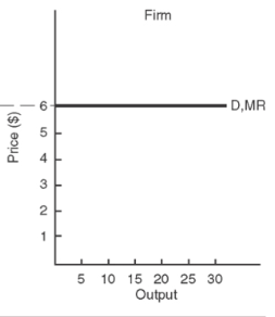
• Competitive market has no control over the price, which is set by the market demand and supply of the good

  • Firm is the price taker and takes the price as “given”

Total and Marginal Revenue

• Total revenue (total sales) → the price of the good times the quantity sold

  • TR = ($ of good)(# of good sold at MC =MR)

• Marginal Revenue → Additional revenue earned by the firm for each additional unit of output sold

  • Marginal Revenue = Equilibrium price (Pe)

Profit Maximization Rule

• As long as Marginal cost is less than marginal revenue, it make sense for the firm to produce the additional unit

  • Marginal cost = (change in total cost) / (change in quantity)

• To maximize profit, produce that quantity, Q, where MR = MC

Short-Run Decision Making of Perfectly Competitive Firm

Firm is making positive economic profits

• the profit maximization rule pridce that quantity where MR=MC

  • Leads to a quantity where MR = MC is greater than the dollar amount on the average total cost (ATC) curve for the same quantity

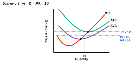
Firm is making a lost, but continues to produce (operate)

• MR =MC at a quantity of 60 units, and for the 60 units, the average total cost (ATC) of producing each unit is $5 which is greater than Pe and MR

  • Firm is making loss but will continue to run its operations and produce because the loss is less than the fixed costs the firm would have to pay if it produced zero output

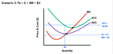
• Firm is making a loss, and decides not to produce at all

  • MR =MC at 40 units, and at this quantity, the fixed costs are greater than the losses that the firm would incur if it produced the 40 units

  

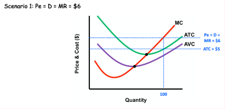
Garlic Market

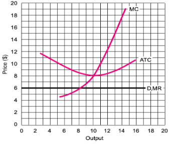
• Market equilibrium price ,Pe = $6

• MC curve starts at about 5 units, MC about $4.50 while MR = $6

  • MR > MC and the garlic producer is making $1.50

    ($6 - $4.50)

  • At *th bushel, MR = MC and ECONOMIC PROFIT IS 0

• TR = $6 × 8 bushel = $48

• TC → using ATC curve

  • 8 bushels, ATC = $8.50

  • TC = $8.50 × 8 bushels = $68

• Profit = TR - TC

  • $48 = $68 = -$20 ($20 loss)

Long-run Outcomes of Perfectly Competitive

Transition to long run for firms making profits int he short run

• Firm making profit but no barriers to entry/exit in perfect competition,

  • These positive economic profits will attract other firms into the industry.

• More firms enter the market → the market supply curve will rise and shift right

  • Leads to a decrease in the market equilibrium price, Pe.

• Firm already in the industry, their profit will fall as Pe falls

• Firm contitue enter the industry until market supply curve shifts far enough to the right,

  • Pe falls to a dollar amount equal to the bottom of the ATC curve

    • Firms in the industry are breaking even and make ZERO ECONOMIC PROFIT

Transition to long run for firms making losses in the short run

• Firm has the option to leave the industry

  • As firm leave the industry, market supply curve will fall and shift to the left

    • lead to an increase in market equilibrium price, Pe.

• Firms remaining in the industry, their losses will be reduced as Pe rises

  • Firms remaining in the industry, their losses will be reduced as Pe rises

• Firm will continue exit the industry until the market supply curve shifts far enough to the left

  • Pe falls to a dollar amount equal to the bottom of the ATC curve

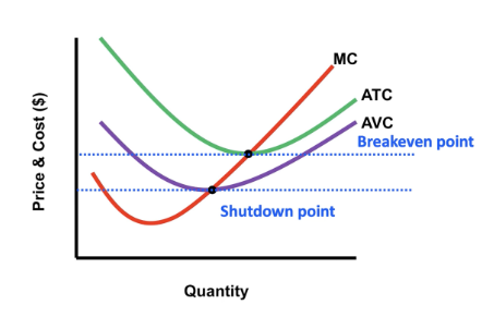
Breakeven and Shutdown Points

• Breakeven point → where MR=MC at bottom of ATC curve

  • FIrm is breaking even, making ZERO ECONOMIC PROFIT (but making a positive normal accounting profit)

  • Firms will be producing the goods at the lowest per unit cost possible

• Shutdown point → where MR=MC at bottom of AVC curve

  • Firm’s losses when it is producing that level of output will be equal tot he fixed cost if the firm were to shutdown operations and produce zero output

  • Pe falls below the price at the shutdown point

    • Firm will shutdown its operations in SHORT RUN

  • In LONG RUN, firm can leave the market if it making losses in the short run

    • A firm that has shutdown its operations would definitely choose not to stay

  • If a firms is operating where MR=MC below the breakeven point and is making losses that are less than its fixed costs,firmsm will also leave the business

Perfect Competition as the “Ideal” Market Structure

• Producing at lowest-cost

  • Firms in perfect competition will be operating at the bottom or minimum of the ATC curve in the long run

    • Breakeven point for the firm, represents the lowest per unit cost of producing that good

    • The point of greatest productive efficiency

  • In long run, perfect competition will lead to firms producing at the lowest cost possible for society as a whole

• Marginal cost pricing

  • Perfect ocmpetition ensures that the price paid by the consumer reflects the “true” cost of producing the last unit of that good

    • “true” cost —> referring to the opportunity costs of producing the good

  • A perfectly competitive firm takes Pe as given and produces where Pe = MR =MC

    • Then Pe= MC which is marginal cost pricing where the price reflects society’s marginal cost of producing the good

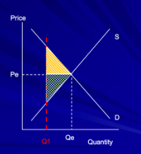
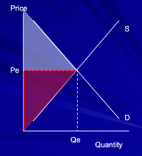
• Maximization of social surplus

  • Consumer surplus → the difference between the price consumers are willing and able to pay for a good and the price they actually pay, Pe.

    • Purple triangle above Pe and to the left of Qe

  • Producer surplus → the difference between the price the producer was willing to accept

    • Red triangle below Pe and to the left of Pe

    

• Deadweight loss → the market instead produced at a quantity less than Qe

  • Consumers would have lost a potential gain in consumer purplus equivalent to the small yellow triangle above Pe and between Q1 and Qe

  • Producers would lose a potential gain in producer surplus equivalent to the small green triangle below Pe and between Q1 and Qe