AP_Microeconomics Unit 3 Notes

3.1 Production Function:

Definition: Relationship between the quantity of inputs and the maximum output produced, assuming efficient techniques. Represented as $Q = f(L, K)$ , where Q is output, L is labor, and K is capital.

Types of Inputs:

Fixed Input: Quantity cannot be varied in the short run (e.g., capital, plant capacity).
Variable Input: Quantity can be varied at any time (e.g., labor, raw materials).

Short vs. Long Run:

Short Run: Period where at least one input is fixed; output adjusted only via variable inputs.
Long Run: Period where all inputs are variable; plant capacity and technology can be altered.

Measuring Production:

Total Product (TP): Total output from a given set of inputs.

Marginal Product (MP): Additional output from one more unit of a variable input; calculated as $MP_L = \frac{\Delta TP}{\Delta L}$ .

Average Product (AP): Average output per unit of variable input; calculated as $AP_L = \frac{TP}{L}$ .

Specialization and Law of Diminishing Returns:

Specialization: Initially, MP increases as variable inputs are added, enhancing efficiency.

Law of Diminishing Returns: As successive units of a variable input are added to a fixed input, beyond a certain point, the marginal product of the variable input will eventually decrease. This happens due to over-utilization of the fixed input.

Production Graphs:

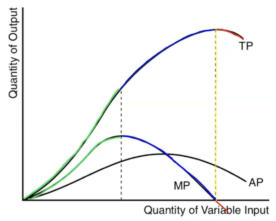
Graph Analysis:

MP and TP Relationship:

MP increasing means TP increases at an increasing rate (Green).
MP positive but decreasing means TP increases at a decreasing rate (Blue).
MP zero means TP is at maximum (Yellow line).
MP negative means TP is decreasing (Red).

MP and AP Relationship:

When MP > AP, AP is rising.
When MP < AP, AP is falling.
When $MP = AP$ , AP is at its maximum (the MP curve intersects the AP curve at AP's maximum).

3.2 Short-Run Production Costs:

Fixed Cost (FC): Costs not varying with output; incurred even at zero output (e.g., rent). Graphically, FC is a horizontal line.

Variable Cost (VC): Costs varying directly with output; zero if no output (e.g., wages for production workers). Graphically, VC starts at the origin and rises, typically increasing at a decreasing rate initially due to specialization, then at an increasing rate due to diminishing returns.

Total Cost (TC): $TC = FC + VC$ . Graphically, the TC curve has the same shape as the VC curve but starts at the FC level on the y-axis.

Marginal Cost (MC): Additional cost of one more unit of output; calculated as $MC = \frac{\Delta TC}{\Delta Q} = \frac{\Delta VC}{\Delta Q}$ .

Average Fixed Cost (AFC): $AFC = \frac{FC}{Q}$ ; declines continuously as output increases (downward sloping curve).

Average Variable Cost (AVC): $AVC = \frac{VC}{Q}$ ; typically U-shaped, reflecting the initial benefits of specialization and then the impact of diminishing returns.

Average Total Cost (ATC): $ATC = \frac{TC}{Q} = AFC + AVC$ ; typically U-shaped, influenced by both the declining AFC and the U-shaped AVC.

Short-Term Production Cost Graph:

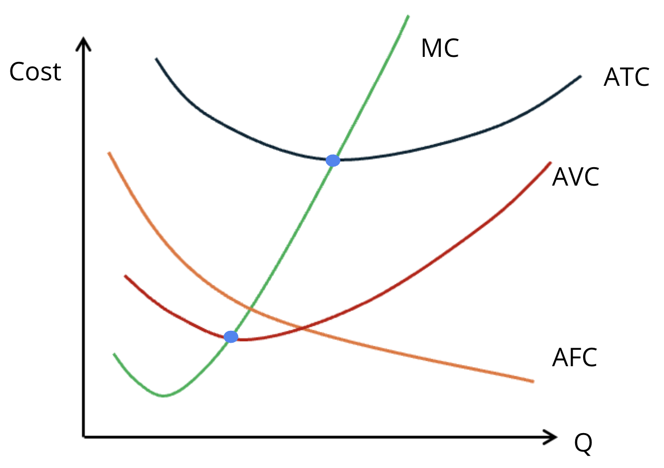
Graph Analysis:

MC (Green):

Initially decreases (specialization).
Eventually increases (diminishing returns).

AFC (Orange):

Decreasing at a decreasing rate.

AVC (Red) and ATC (Blue) Relationship:

Both are U-shaped
AFC is always decreasing, so AVC and ATC get closer together.

MC (Green) and AVC and ATC Relationship:

The MC curve intersects both the AVC and ATC curves at their minimum points.
When MC is below AVC or ATC, they’re decreasing.
When MC is above AVC or ATC, they’re increasing.

3.3 Long-Run Production Costs:

Long-Run Average Total Cost (LRATC): Shows the lowest average cost for any output level when all inputs are variable. Graphically, the LRATC curve is an envelope of many short-run average total cost (SRATC) curves, each representing a different plant size.

Returns to Scale:

Refers to the technical relationship between input and output, describing how output changes when all inputs are increased proportionally:

Increasing Returns: Output more than doubles (>2x) when all inputs double (2x).
Constant Returns: Output doubles (=2x) when all inputs double (2x).
Decreasing Returns: Output less than doubles (<2x) when all inputs double (2x).

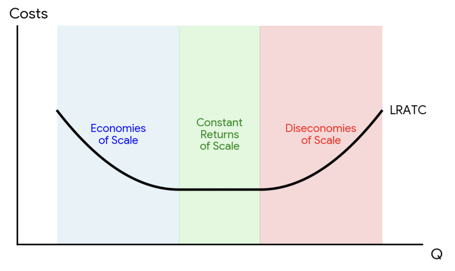
Economies of Scale and Diseconomies of Scale:

Economies of Scale: Represent the cost advantages a firm experiences as it increases its scale of production. These lead to lower long-run average costs (LRAC falls). This typically occurs in situations characterized by increasing returns to scale.

Graph Analysis: Graphically, economies of scale are depicted by the downward-sloping portion of the LRAC curve.

Diseconomies of Scale: Represent the cost disadvantages (higher average costs) a firm experiences when it expands its scale of production beyond an optimal point. These lead to higher long-run average costs (LRAC rises). This typically occurs in situations characterized by decreasing returns to scale.

Graph Analysis: Graphically, diseconomies of scale are depicted by the upward-sloping portion of the LRAC curve.

Constant Returns to Scale in a Cost Context: If output doubles when all inputs double, the long-run average cost (LRAC) remains constant. This is represented by a flat portion of the LRAC curve.

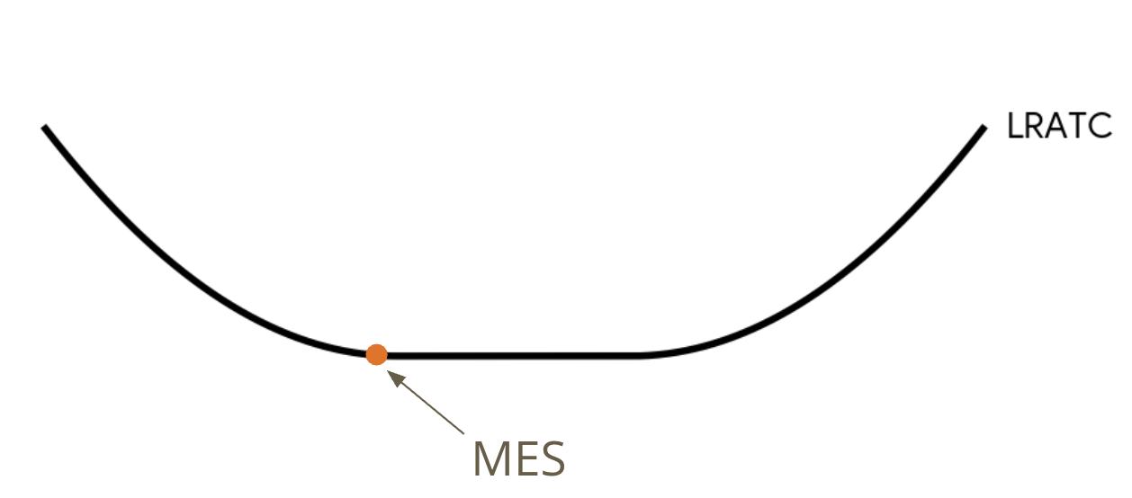
Minimum Efficient Scale (MES): Lowest output level where a firm achieves the lowest possible long-run average cost. Graphically, this is the point where the LRAC curve reaches its minimum.

3.4 Types of Profit:

Accounting Profit: Total Revenue - Explicit Costs (out-of-pocket expenses).

Economic Profit: Total Revenue - Explicit Costs - Implicit Costs (opportunity costs).

Normal Profit: Economic profit = 0; firm covers all explicit and implicit costs, representing the minimum to stay in business.

3.5 Profit Maximization:

Goal: Maximize profit by producing where $MR = MC$ (Marginal Revenue equals Marginal Cost).

If MR > MC, produce more; if MR < MC, produce less.

Perfect Competition: Price equals marginal revenue ( $P = MR$ ), so profit maximization occurs where $P = MC$ .

Shutdown Rule (Short Run): Produce if $P \ge AVC$ to cover variable costs and some fixed costs; shut down if :P < AVC

Exit Rule (Long Run): Exit the industry if P < ATC (firm is making negative economic profit).

3.6.1 Firm's Short-Run Decision to Produce and Long-Run Decision to Enter or Exit a Market:

In the short run, a firm must decide whether to continue production or shut down temporarily, given that at least one resource (e.g., factory size) is fixed. Fixed costs must be paid regardless of production. The critical factor is whether the firm can cover its variable costs.

Scenario 1: Produce
- Condition: Price ( $P$ ) > Average Variable Cost ( $AVC$ ).
- Explanation: If the market price covers variable costs, the firm's total revenue will exceed its variable costs, allowing it to continue operations. Production helps minimize losses on fixed costs, as these costs are incurred irrespective of output.
Scenario 2: Shut Down
- Condition: Price ( $P$ ) < Average Variable Cost ( $AVC$ ).
- Conclusion: It is more cost-effective for the firm to shut down temporarily to avoid incurring losses that would exceed its fixed costs.

The decision can also be analyzed using total or per-unit measurements:

Total Measurement:
- If Total Revenue ( $TR$ ) > Total Cost ( $TC$ ): The firm is profitable and should continue production.
- If $TR = TC$ : The firm breaks even.
- If TR < VC < TC: The firm should shut down temporarily.
- Shutdown Rule: TR < VC.
Per Unit Measurement:
- Production always occurs where Marginal Revenue ( $MR$ ) = Marginal Cost ( $MC$ ), provided $P \ge AVC$ .
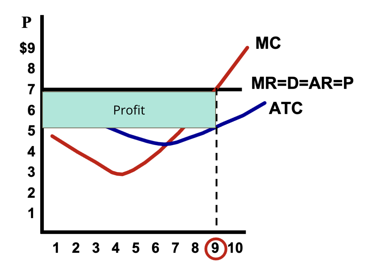
- If MR > ATC: Firm is making a profit.
- If $MR = ATC$ : The firm breaks even (earns normal profit).
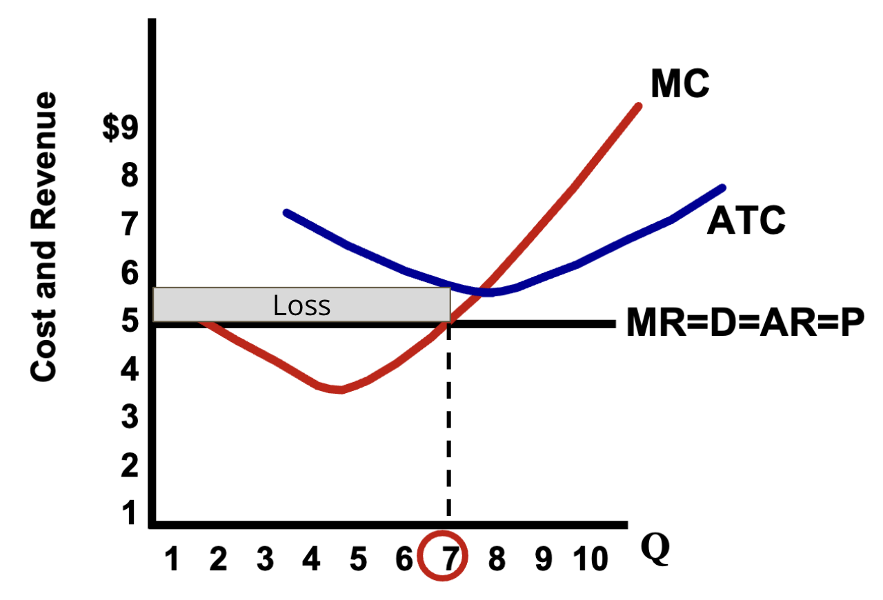
- If ATC > MR \ge AVC: The firm operates at a loss but should still produce to cover variable costs and contribute to fixed costs.
- If MR < AVC: The firm should shut down temporarily.
- Shutdown Rule: MR < AVC (equivalent to P < AVC in perfect competition).

Short-term Production Cost Graph:

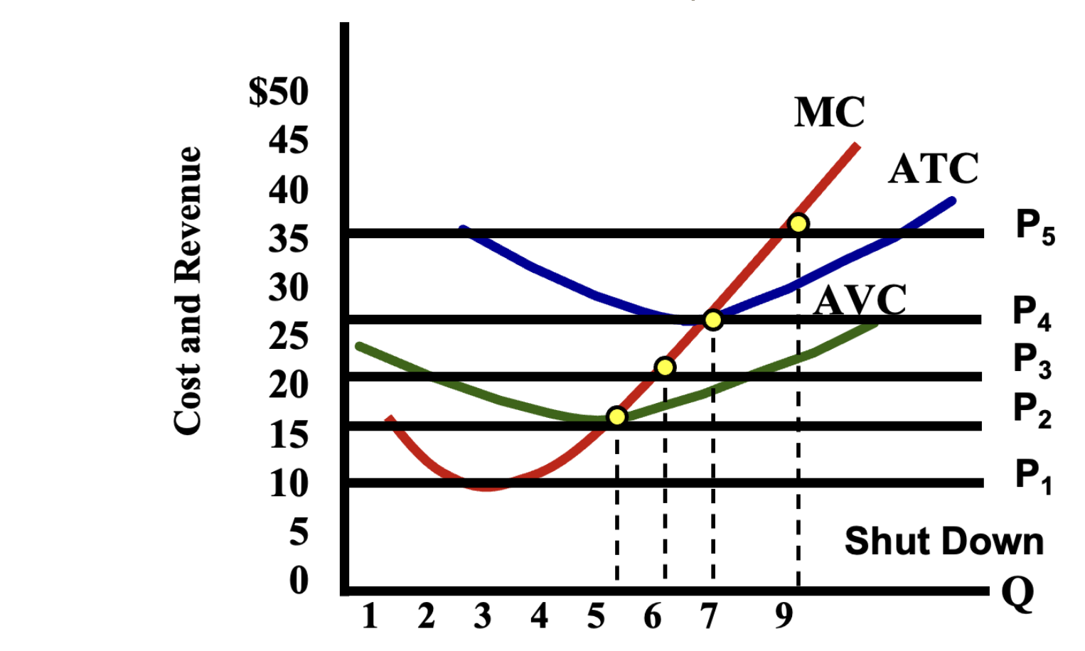
Graph Analysis:

Shut Down:
- P1: MC < AVC
- P2: MC = AVC
  - Shut Down Rule: When MR = MC < AVC
Continue Production:
- P3: AVC < MC < ATC - Operating at a Loss
- P4 MC = ATC - Breaking Even
- P5 MC > ATC - Positive Economic Profit

Marginal Cost and Short-Run Supply:

Firms maximize profit by producing where price equals marginal cost ( $P = MC$ ).
The marginal cost curve above the average variable cost ( $MC \ge AVC$ ) represents the firm’s short-run supply curve.

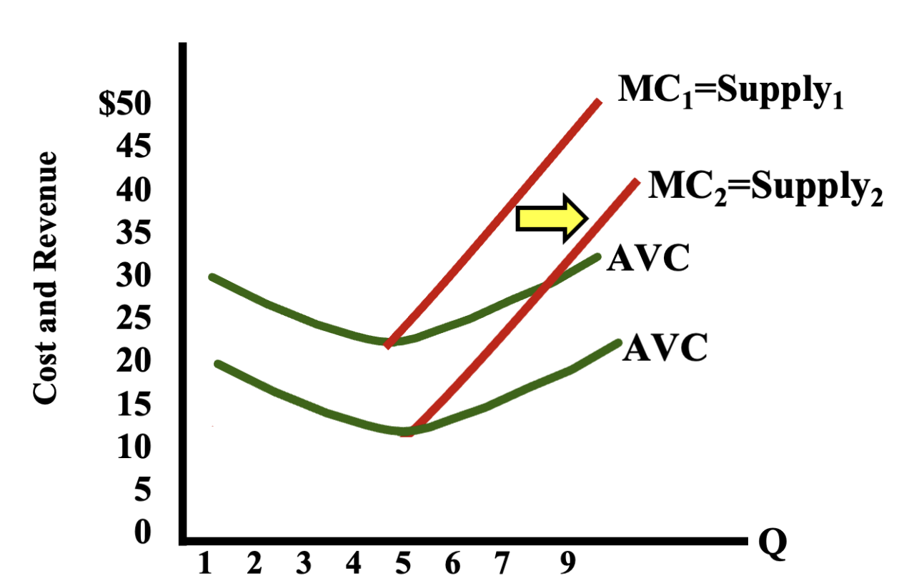
Effects of Changes in Variable Costs:

When variable costs increase (e.g., per unit tax), the marginal cost curve shifts upward, leading to a decrease in supply.

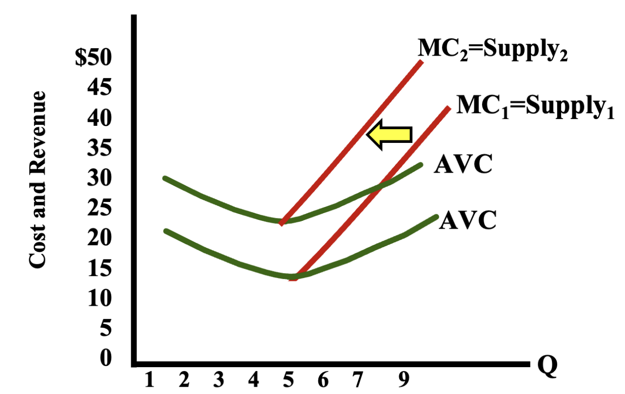
When variable costs decrease (e.g., subsidy), the marginal cost curve shifts downward, leading to an increase in supply.

3.6.2 Firm's Long-Run Decision to Enter or Exit a Market:

In the long run, all inputs are variable, allowing firms to adjust their size and capacity or to enter/exit an industry in response to market conditions.

Scenario 1: Enter
- Condition: Price ( $P$ ) > Average Total Cost ( $ATC$ ).
- Explanation: The firm can make economic profits, the price covers all explicit and implicit costs.
- Conclusion: Firms enter the market, increasing market supply.
Scenario 2: Exit
- Condition: Price ( $P$ ) < Average Total Cost ( $ATC$ ).
- Explanation: The firm has persistent economics losses, the price is too low to all explicit and implicit costs.
- Conclusion: Firms exit the market permanently, decreasing market supply.

Economic Profit and Market Dynamics:

Firms enter markets to secure economic profits and exit to avoid economic losses. This movement drives perfectly competitive markets towards a long-run equilibrium where economic profit is zero and $P = ATC$ .

Barriers to Entry and Profit:

Barriers to Entry: Factors hindering new firms from entering a market (e.g., capital requirements, regulatory restrictions).
Low barriers lead to more competition and lower individual profits.
High barriers lead to less competition and higher individual profits.

Normal Profit in Competitive Markets:

In perfectly competitive markets, firms achieve a normal profit (Economic Profit = 0 )in the long run, meaning they cover all explicit and implicit costs but do not generate additional profit beyond that necessary to remain in business - $P = ATC$ .

3.7 Perfect Competition:

Perfect Competition Details:

Key Characteristics:
- A large number of small firms with identical products (perfect substitutes).
- Absence of barriers allows free market entry and exit.
- Firms have no incentive to advertise and are price takers.
Price Taker Behaviour:
- Firms operate as price takers; if one firm raises its price above market standards, it will lose all customers to competitors.
- Demand Graph for an Individual Firm in Perfect Competition:
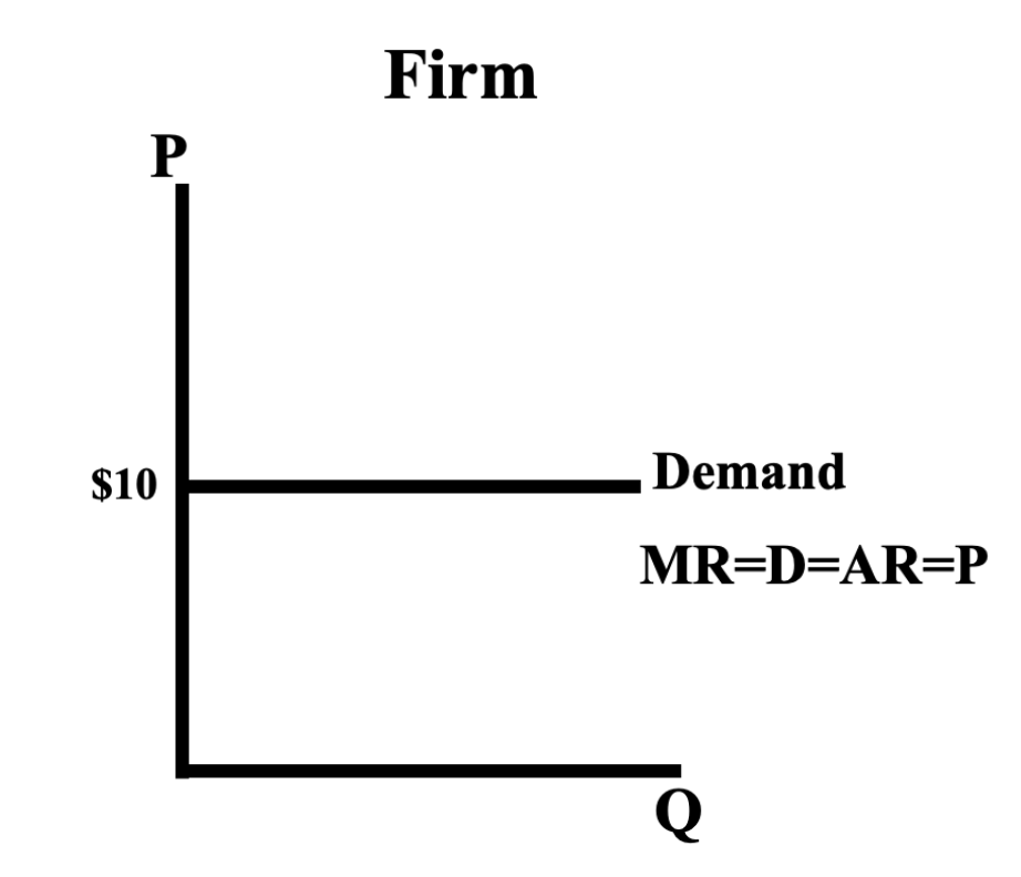
- The demand curve for an individual firm in perfect competition is perfectly elastic, represented by a horizontal line at the market price.
Revenue in Perfect Competition:
- The additional revenue from selling an additional unit remains constant: $MR=D=AR=P$ (where $MR$ is marginal revenue, $D$ is demand $AR$ is average revenue, and $P$ is the price).

Profit and Loss Calculation:

Analysis of Profit or Loss:
- Total Revenue ( $TR$ )
- Total Cost ( $TC$ )
- Profit/Loss = $TR - TC$
- When TR>ATC the firm earns profit (positive economic profit).
- When TR<ATC the firm suffers a loss (negative economic profit).

General Rules:

Shut Down Rule: If P<AVC : shutting down and covering FCs incurs less losses than staying open and covering TCs.

Profit Maximization Rule: $MR = MC$ applies across all market structures as long as P>AVC .
For perfectly competitive firms, this simplifies to $P = MC$ since $P=MR$ .

3.8.1 Important Formulas:

Production Function: $Q = f(L, K)$
Marginal Product: $MP_L = \frac{\Delta TP}{\Delta L}$
Average Product: $AP_L = \frac{TP}{L}$
Total Cost: $TC = FC + VC$
Marginal Cost: $MC = \frac{\Delta TC}{\Delta Q} = \frac{\Delta VC}{\Delta Q}$
Average Fixed Cost: $AFC = \frac{FC}{Q}$
Average Variable Cost: $AVC = \frac{VC}{Q}$
Average Total Cost: $ATC = \frac{TC}{Q} = AFC + AVC$
Accounting Profit = Total Revenue - Explicit Costs
Economic Profit = Total Revenue - Explicit Costs - Implicit Costs
Total Profit: $Profit = TR - TC$
Revenue in Perfect Competition: $MR = AR = P$
Short-Run Shutdown Rule (Total Revenue): TR < VC
Short-Run Shutdown Rule (Per-Unit): P < AVC or MR < AVC
Long-Run Exit Rule (Per-Unit): P < ATC or MR < ATC

3.8.2 Concepts/Rules:

Law of Diminishing Returns: Adding more of a variable input to a fixed input eventually decreases its marginal product.
Profit Maximization Rule: Always occurs where Marginal Revenue ( $MR$ ) = Marginal Cost ( $MC$ ), provided the price covers variable costs.
Perfect Competition Profit Maximization: Produce where $P = MR = MC$ .
Short-Run Shutdown Rule: Continue production if $P \ge AVC$ ; shut down if P < AVC.
Long-Run Exit Rule: Exit the industry if P < ATC.
Short Run vs. Long Run:
- Short Run: Period where at least one resource (e.g., factory size) is fixed. Firms cannot change capacity.
- Long Run: Period where all resources are variable. Firms can adjust their size and capacity.
Short-Run Production Decision (Produce or Shut Down):
- Produce: If Price ( $P$ ) > Average Variable Cost ( $AVC$ ). The firm covers variable costs and contributes to fixed costs.
- Shut Down Temporarily: If P < AVC. Losses would exceed fixed costs if production continued.
Long-Run Market Decision (Enter or Exit):
- Enter: If Price ( $P$ ) > Average Total Cost ( $ATC$ ). Firms make economic profits, attracting new entrants.
- Exit: If P < ATC. Firms experience persistent economic losses and leave the market.
Perfect Competition Characteristics: Many small firms, identical products, no barriers to entry/exit, firms are price takers ( $P = MR = AR$ ). In the long run, perfect competition leads to a normal profit (zero economic profit) where $P = ATC$ .
Barriers to Entry: Factors that make it difficult for new firms to enter an industry, influencing competition and profitability.