Data Structures list
This guide breaks down essential data structures for C/C++ developers, designed to make them easy to understand and directly applicable to technical interviews (like NeetCode/LeetCode). We have included real-world analogies, concise explanations, essential time complexities, illustrative C/C++ code, and clear diagrams for every single structure.
1. Dynamic Arrays (Vectors)
The Concept: A dynamic array is like a contiguous row of lockers. You can add lockers to the end as needed. When you run out of space, the system automatically buys a whole new, larger block of lockers elsewhere, copies everything over, and destroys the old, smaller row.
[Image 0: Diagram illustrating the dynamic array memory reallocation process]
Real-World Example: Think of assigned seating in a theatre. If your entire family (a set of data) needs to sit together, you buy a consecutive block of seats. If more family members arrive and the current row is full, the entire family must move to a completely new, longer row where you can all fit together again.
C/C++ Implementation Example (std::vector):
C++
#include <iostream>
#include <vector>

int main() {
    // 1. Creation: A vector of integers (dynamic array)
    std::vector<int> myVector;

    // 2. Operation: Adding elements (O(1) amortized)
    myVector.push_back(10);
    myVector.push_back(20);
    myVector.push_back(30);

    // 3. Operation: Accessing an element (O(1))
    std::cout << "Element at index 1: " << myVector[1] << std::endl; // Output: 20

    // 4. Operation: Size of the vector
    std::cout << "Vector size: " << myVector.size() << std::endl; // Output: 3

    return 0;
}
Time Complexity:
Access (Index): O(1)
Insertion/Deletion (at end): O(1) amortized (O(N) during reallocation)
Insertion/Deletion (in middle/front): O(N) (due to shifting elements)
C/C++ Context: In C++, this is std::vector. This is the go-to default sequence container because it stores elements in contiguous memory. This makes vectors incredibly cache-friendly and fast for access, but very slow for inserting/deleting elements anywhere except the very end.
2. Singly Linked Lists
The Concept: A linked list is like a chain or a sequence of clues in a scavenger hunt. Each node (clue) contains a value and the precise memory location (a pointer) of the next clue in the chain. You cannot skip clues; you must follow them in order from the start (the Head) to find the end.
[Image 1: Batch diagram showing Singly Linked List (with Head/NULL pointers), Hash Table (with collision handling), and Binary Search Tree (with sorting rule)]
Real-World Example: A train is a perfect analogy. The locomotive is the Head. Each train car is a node. To get to the 10th car, you must walk through cars 1 through 9. Each car is connected only to the cars immediately before and after it.
C/C++ Implementation Example (std::forward_list or raw pointers):
C++
#include <iostream>

#include <forward_list> // STL for Singly Linked List

// Basic raw pointer Node definition (conceptual)

struct Node {

int data;

Node* next;

};

int main() {

// 1. Creation: A singly linked list (STL version)

std::forward_list<int> myList;

// 2. Operation: Insertion at the front (O(1))

myList.push_front(30);

myList.push_front(20);

myList.push_front(10); // List is now 10 -> 20 -> 30

// 3. Operation: Iteration (O(N))

std::cout << "Linked List: ";

for (int value : myList) {

std::cout << value << " -> ";

}

std::cout << "NULL" << std::endl;

return 0;

}
Time Complexity:
Access (Index): O(N)
Insertion/Deletion (at Head): O(1)
Insertion/Deletion (in middle): O(1) if you already have the pointer to that specific node.
C/C++ Context: The STL provides std::forward_list (singly) and std::list (doubly linked). Linked lists are not contiguous in memory, meaning they have poor cache locality but are excellent when you need constant-time insertion/deletion anywhere in the structure, provided you are already pointing to that spot.
3. Hash Tables (Hash Maps)
The Concept: A hash table is like a highly efficient filing cabinet system. You provide a Unique "Key" (e.g., a person's name). A "Hash Function" scrambles that name into a single integer. This integer is used as an exact index to directly open one of the filing cabinet's buckets (an underlying array) and instantly access the "Value" (the person's file) without looking through any other drawers.
Real-World Example: A dictionary is a hash table. The word you want to look up is the Key. The alphabetical order of the words effectively serves as the "Hash Function" that guides you instantly to the specific page (the Value) where that word's definition is stored.
C/C++ Implementation Example (std::unordered_map):
C++
#include <iostream>

#include <string>

#include <unordered_map> // STL for Hash Map

int main() {

// 1. Creation: Map from student Name (string) to ID (int)

std::unordered_map<std::string, int> studentIds;

// 2. Operation: Insertion (Key-Value pairs) (O(1) average)

studentIds["Alice"] = 101;

studentIds["Bob"] = 102;

studentIds["Charlie"] = 103;

// 3. Operation: Accessing/Searching (O(1) average)

std::cout << "Bob's ID: " << studentIds["Bob"] << std::endl; // Output: 102

// 4. Operation: Check for key existence (O(1) average)

if (studentIds.find("Dave") == studentIds.end()) {

std::cout << "Dave not found in map." << std::endl;

}

return 0;

}
Time Complexity:
Search/Access/Insertion/Deletion: O(1) average. O(N) worst-case (if many keys hash to the same bucket).
C/C++ Context: Use std::unordered_map (for key-value pairs) or std::unordered_set (for storing unique keys). These containers manage dynamic hashing and collision handling (often using chaining, shown in the diagram above) for you.
4. Binary Search Trees (BST)
The Concept: A BST is a tree-like hierarchy that organizes sorted data. It always starts at a Root node. Every node has up to two children. It follows one non-negotiable rule: all values in the entire left subtree must be smaller than the parent, and all values in the entire right subtree must be larger.
Real-World Example: Looking for a phone number in a sorted digital directory is a BST operation. You choose the middle letter of the alphabet (the Root, e.g., 'M'). If the name starts with 'B', you instantly ignore the entire right side ('N' through 'Z') and repeat the process on the left side until you find the name.
C/C++ Implementation Example (std::set or raw pointers):
C++
#include <iostream>

#include <set> // STL equivalents are balanced BSTs

// Basic raw pointer Node definition (conceptual)

struct TreeNode {

int val;

TreeNode* left;

TreeNode* right;

};

int main() {

// 1. Creation: A set (implemented as a self-balancing BST)

std::set<int> mySet;

// 2. Operation: Insertion (O(log N))

mySet.insert(50);

mySet.insert(30);

mySet.insert(70);

mySet.insert(20);

mySet.insert(40);

// 3. Operation: Search/Existence (O(log N))

if (mySet.count(30)) {

std::cout << "30 is in the tree." << std::endl;

}

// 4. Operation: Automatic sorted iteration (O(N))

std::cout << "Sorted elements: ";

for (int value : mySet) {

std::cout << value << " ";

}

// Output: 20 30 40 50 70

std::cout << std::endl;

return 0;

}
Time Complexity:
Search/Access/Insertion/Deletion: O(log N) average. O(N) worst-case (if the tree is highly unbalanced, like a linked list).
C/C++ Context: The STL containers std::set, std::multiset, std::map, and std::multimap are typically implemented as Red-Black Trees, which are a specialized type of self-balancing BST. This guarantees O(log N) operations by ensuring the tree never becomes too skewed.
NeetCode/LeetCode Data Structure Cheat Sheet
This section covers the remaining crucial data structures you will need for algorithmic problems. Master these STL containers to solve NeetCode/LeetCode challenges efficiently.
C/C++ STL & Complexity Summary:
[Image 2: Batch diagram showing Stack (LIFO), Queue (FIFO), and Priority Queue (Max Heap)]
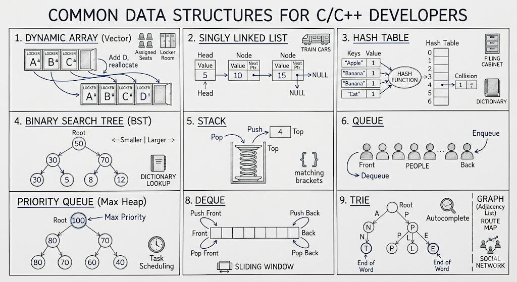
1. Stack: LIFO (Last-In, First-Out). Elements are added and removed only from the top.
STL: std::stack<T>
Complexity: Push/Pop: O(1). Top/Empty: O(1).
2. Queue: FIFO (First-In, First-Out). Think of a physical line of people. Elements are added to the back (Enqueue) and removed from the front (Dequeue).
STL: std::queue<T>
Complexity: Enqueue/Dequeue: O(1). Front/Back: O(1).
3. Priority Queue (Heap): A tree structure where the element with the highest (or lowest) priority is always at the Root. Perfect for finding 'Top K' elements.
STL: std::priority_queue<T> (Default is a Max Heap, where largest is top). Use std::priority_queue<int, std::vector<int>, std::greater<int>> for a Min Heap.
Complexity: Push/Pop (Insert/Extract): O(log N). Top: O(1).
[Image 3: Batch diagram showing Deque (Double-Ended Queue operations), Trie (Prefix Tree with 'APPLE'/'ANTS'), and Graph representation as an Adjacency List]
4. Deque (Double-Ended Queue): A sequence that allows constant-time insertion and deletion at both the front and the back. Used often for sliding window problems.
STL: std::deque<T>
Complexity: Push/Pop (both ends): O(1). Random Access: O(1).
5. Trie (Prefix Tree): A specialized tree for storing strings. The nodes represent characters, and paths from the root form words. Crucial for autocomplete, spellcheck, and complex string problems.
STL: No direct STL equivalent. You must build this using custom struct TrieNode.
Complexity: Insert/Search: O(L), where L is the length of the string. Space: O(ALPHABET_SIZE * N * L).
6. Graph (Adjacency List): A connection of vertices (nodes) and edges (relationships). While graphs can be complex, the most common interview representation is an array of vectors.
C++ Representation: std::vector<std::vector<int>> adjList(numVertices); or std::vector<std::list<int>> adjList(numVertices);.
Complexity (Adjacency List): Add Edge: O(1). Check connection (u, v): O(degree(u)). Find all neighbors of (u): O(degree(u)). Space: O(V + E).