Fiscal policy
The concept of fiscal policy
Fiscal policy refers to the use of Commonwealth Government spending and taxation to affect the level of economic activity and to achieve specific economic and social objectives.
The main economic objectives of the government include economic growth, full employment and price stability.
Fiscal policy first came into prominence during the Great Depression era of the 1930s when most economies suffered from unemployment rates that reached as high as 30% of the workforce.
Prior to 1930s it was considered prudent for the government to simply balance its budget and not interfere with the operation of the market economy.
Since the economy was assumed to operate close to full employment, there was little need for the government to attempt to stabilise the business cycle.
It was British economist, John Maynard Keynes, who was able to show that economies could get stuck in prolonged economic contractions and that the Government, through fiscal policy could stimulate the economy with increased government spending and/or tax cuts.
The ‘Keynesian Revolution’ was born based on the premise that aggregate demand was the most important driving force of the economy and that fiscal policy could be used to smooth the business cycle.
The fiscal policy operates through the Government’s annual Budget Statement setting out its main priorities and its estimates for expenses (spending) and revenue.
Government expenses can be divided into three broad categories:
Government purchases of goods and services accounts for around 60% of government spending. This includes spending in areas such as health, education, defence and general public services.
An increase in government purchases will directly increase aggregate demand and increase real GDP and employment.
Government investment accounts for around 4 per cent of the government’s spending. This includes spending on public infrastructure such as transport, including roads and bridges and public buildings such as schools and hospitals.
An increase in government investment will directly increase aggregate demand and increase real GDP and employment. It will also increase aggregate supply by adding to the nation’s capital stock.
Government transfer payments accounts for around 37 per cent of
government spending. This includes spending on social security and
welfare payments including the age pension, disability payments
and unemployment benefits.
An increase in transfer payments will increase household disposable income and increase consumption expenditure which will then increase real GDP.
Government taxation can also be divided into three main categories:
Personal income tax is a progressive tax levied on wage and salary earners. It is the Government’s main source of income accounting for 47 per cent of the Government’s total revenue.
An increase in income tax rates will decrease consumption expenditure, shifting the aggregate demand (AD) curve to the left, decreasing real GDP and employment. An increase in income taxes may also affect the aggregate supply (AS) curves because it may reduce workers’ incentive to supply labour and therefore decrease aggregate supply.
Company tax is a flat rate tax levied on company profits. It accounts for 20 per cent of the Government’s revenue.
An increase in the company tax rate will reduce corporate profits and decrease business investment, shifting the AD curve to the left, decreasing real GDP and employment.
Consumption taxes (the GST and excise duties) are indirect taxes levied on goods and services. These taxes account for around 20 per cent of the Government’s revenue.
An increase in these taxes will decrease consumption expenditure which will then decrease aggregate demand.
Fiscal policy can have a powerful effect on the level of economic activity because it can directly affect the government purchases component in aggregate demand and indirectly affect the consumption and investment components through taxes and transfer payments.
The Government’s policy objectives
The four most important macroeconomic policy objectives for the Australian' government are:
Sustainable economic growth
Full employment (low unemployment)
Price stability (low inflation)
Reduced income inequality
Sustainable economic growth
Economic growth occurs when potential GDP increases.
It can be illustrated by a shift of either the economy’s production possibility frontier (PPF) to the right or the economy’s long run aggregate supply curve to the right.
Economic growth means that there has been an increase in the productive capacity of the economy and is usually measured by an increase in real gross domestic product (real GDP) over time.
If population grows faster than output then living standards fall so economists tend to focus on change in real GDP per capita.
What does sustainable economic growth mean?
Sustainable means balancing economic growth with environmental and social considerations such as healthcare and social equity to improve long-term prosperity.
Pursuing sustainable growth means we can improve current living standards without compromising the living standards of future generations.
What should be the target growth rate for the economy?
The government should aim for real GDP to match the growth in potential GDP. Each year potential GDP increases by between 2.5-3% which is driven by growth in the labour force and productivity.
If actual growth is less than this then unemployment will increase, if growth exceeds this rate, then inflation and the cost of living will rise.
Our growth rate has averaged 2.7% while real GDP per capita has increased at an annual rate of 1.2%.
What is the most important determinant of economic growth?
Output will always grow by simply increasing the quantity of resources, such as the labour force and/or capital stock. But GDP per capita will only increase if labour productivity increases.
Full employment
Full employment refers to the situation where everyone who is willing and able to work can find a job.
There are two types of unemployment that are always present in the labour market:
Frictional - often referred to as ‘search unemployment’, occurs when people first enter the workforce or when people voluntarily quit their current job to search for a new job. Typically between 1.5-2.5% of the workforce
Structural - occurs if there is a mismatch of available required skills for a particular geographical or occupational sector of the economy. Typically between 1.5-2.5% of the labour force
The sum of frictional and structural unemployment is equal to the natural rate of unemployment. For Australia, the natural rate of unemployment is estimated to be around 4% and this is the standard definition of full employment used by most economists.
Cyclical unemployment is when the economy’s growth rate slows or contracts so that the actual real GDP is less than potential GDP. In other words, is unemployment increases quite rapidly when the economy is in recession and experiences a negative output gap.
When cyclical unemployment is zero this is when the economy is fully employed.
The RBA defines full employment as the maximum level of employment that is consistent with low and stable inflation.
The RBA prefers to use the NAIRU - the non accelerating inflation rate of unemployment below which wage inflation begins to accelerate, indicating tightness in the labour market.. The estimate of NAIRU is around 4.5%
The Australian economy experienced full employment conditions between 2022 and 2024 when the unemployment rate fluctuated between 3.5 and 4.2%.
Achieving a low unemployment rate close to the natural rate is important because of the significant economic and social costs associated with high unemployment.
There is a direct monetary cost because government welfare payments will increase and at the same time, government tax revenue will fall.
This presents an opportunity cost because this money could be spent on other government provided goods such as education or healthcare.
High rates of unemployment will mean lower consumption spending which will have a negative impact on business confidence and therefore investment spending.
Lower rates of investment will reduce future economic growth which means that average living standards will potentially lower. Long term unemployment also imposes considerable personal and social costs on those who cannot find work affecting both their mental and physical health.
Price stability
Price stability means maintaining a low and stable of inflation over time. This helps maintain the value of money. This ensures that the same quantity of money buys roughly the same amount of goods and services tomorrow as it does today.
The targets for consumer inflation is a rate between 2-3% on average, over the course of the business cycle.
Achieving price stability is important because it avoids the damaging costs of high inflation:
inflation increases the cost of living and erodes the purchasing power of household incomes reducing the living standards of the average household
inflation will cause interest rates to rise, which will adversely affect business investment decisions and household spending on discretionary goods and services
inflation erodes the confidence people have in money as a store of value, so many households seek ‘hedges’ against expected price rises by purchasing assets (e.g. property) which are likely to appreciate in value. Such as speculative activity reduces the potential output of the economy if it diverts resources away from productive investment.
business investment decisions are more risky in an inflationary
environment because rising prices make it more difficult to maintain
costs and operate profitably.
international competitiveness will be adversely affected if domestic
inflation rates exceed those overseas - foreign demand for domestic
goods and services will fall while domestic demand for imported
goods and services will increase.
high inflation will increase income inequality. High income groups
are better able to ‘insulate’ themselves from inflation compared to low
income groups by purchasing assets that rise in value with inflation.
People on fixed incomes such as pensions and other government
transfer payments will see an erosion in the value of their income.
sustained inflation also effects taxation and government revenue. ‘Pay
as you go’ (PAYG) taxpayers suffer bracket creep as inflation gradually causes their income levels to rise to levels where they are liable for higher marginal rates of taxation.
Reducing income inequality
This is about achieving a more equitable distribution of income is an important priority.
The most common measure of inequality is the Gini coefficient, which is derived from the Lorenz curve.
A Lorenz curve plots the cumulative percentage of total income received against the cumulative number of household, starting with the poorest household.
The Gini coefficient measures the extent to which the distribution of income deviates from a perfectly equal distribution. Its value ranges from zero to one, where zero represents perfect equality and one represents complete inequality.
The fiscal policy is particularly well suited to reducing income inequality through its spending and taxing powers. The Commonwealth Government’s main tax is personal income tax which is progressive tax and accounts for nearly half of the Government’s tax revenue.
As income rises, the marginal rate of tax rises which means that higher income groups pay a greater proportion of tax than lower income groups.
The largest category of Commonwealth Government is social security and welfare. This accounts for more than one third of the Government’s budget.
Direct transfer payments (pensions and benefits) provide cash support for a number of groups of Australians - the aged, the unemployment, the sick and disabled, sole parents and families with children family allowance.
Indirect government payments (social transfer in-kind) also redistribute income from the highest earners to the lowest. Public services like education social housing and health are provided at less than their full cost, as they are subsidised by the government. These subsidies help to redistribut income and enable all Australians to have access to basic services. If these services were provided by the market, it is likely that some households would not be able to afford them, so they would be under-consumed. Fewer people would obtain educational qualifications, find housing or be able to seek medical treatment.
Budget outcomes - balanced, surplus or deficit
The outcome of the budget refers to the relationship between government revenue (T) and government expenses (G).
Is government expenses the same as government purchases of goods and services that is recorded in the GDP statistics?
The answer is no because government expenses includes spending on transfer payments which is not included in the ‘G’ component.
When the Government frames its budget each year, there are three possible outcomes:
a balanced budget, where outlays equal revenue (G = T)
a budget surplus, where outlays are less than revenue (G < T). This means that the Government is saving
a budget deficit, where outlays are greater than revenue (G > T). A budget deficit means that the Government is dis-saving and will need to borrow to finance the deficit.
Should the Government always aim for a balanced budget?
No. This is because the Government can use fiscal policy as a means to target its economic objectives.
For example, if the economy contracted and unemployment was rising, then the Government would aim for a budget deficit in order to inject more money into the economy and increase the level of economic activity.
A budget deficit will have an expansionary effect on the economy because it represents a net injection of government spending. If the government planned its budget, this would plunge the economy deeper into recession.
If real GDP growth rate was excessive and the economy entered a boom with high inflation, then the Government would aim for a budget surplus in order to withdraw money from the economy and decrease the level of economic activity.
A budget surplus would have a contractionary effect on the economy because it represents a net withdrawal of government spending.
What will be the impact of a balanced budget?
This will have a neutral effect on the level of economic activity because the injection of government spending into the economy will exactly match the withdrawal of revenue.
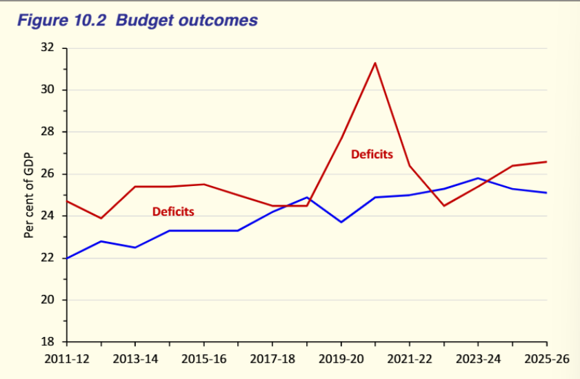
First, the ‘normal’ value for both government expenses and government revenue is between 24 and 26% of GDP.
Second, government spending is more volatile compared with government revenue
Third, for 13 out of 15 years shown in the graph, the budget outcome was a deficit.
It is important to realise that the business cycle can play a major role in affecting the outcome of the budget in any particular year and this is clearly evident from figure 10.2.
In a period of expansion, for example, the government’s tax revenue will increase as employment grows and as firms profits increase. Revenue from the GST and excise duties will also grow as consumer spending rises. At the same time, spending on welfare will decline since unemployment is falling.
When government revenue increases relative to government spending the budget balance will increase - either an existing budget surplus will get bigger or an existing deficit will get smaller.
In a business cycle contraction, the opposite will happen where government tax revenue will fall while government spending on welfare will rise causing the budget balance to fall. Notice the massive spike in government spending during the Covid recession period of 2020-21 resulting in record budget deficits.
The planned budget versus the actual budget outcome
It is almost certain that the actual budget outcome at the end of the financial year will be very different from the planned outcome at the beginning of the year.
While preparing its planned budget the Government has to make assumptions about the expected rate of growth of not only real GDP, but for employment, inflation, unemployment, the exchange rate and commodity prices, to name a few.
If any one of these assumptions is inaccurate, then the Government’s estimates of both revenue and outlays will change over the course of the year.
Suppose there is a downturn in economic activity causing business profits to fall and unemployment to rise. Taxation revenue from both households and businesses would decrease. This would mean that the actual budget balance will decrease compared with the planned budget.
Alternatively, if there was an unanticipated upswing in economic activity after the announcement of the budget, then government revenue would rise while welfare spending would fall, causing the actual budget balance to be higher than forecast.
Changes in the global economy could also impact on the budget outcome. For example, a fall in commodity prices would reduce the government’s actual revenue from both resource royalities and company tax resulting in the actual budget to be lower than forecast.
Economic shocks could also cause the actual outcome to differ significantlly from the predicted result. Events such as bushfires, floods and health crises such as the Covid pandemic could not have been anticipated in the Budget forecasts for the relevant years.
Financing a budget deficit
When the Government records a budget deficit, its expenditure exceed its revenue and therefore it needs to finance the difference.
This is usually achieved through Government borrowing, although it could also raise funds through selling some government assets.
The four main methods a government can use to finance a budget deficit are:
selling new government bonds to domestic residents
selling new government bonds to overseas residents
borrowing from the Reserve Bank
selling government assets
The Government borrows by selling new government bonds, known as Commonwealth Government Securities (CGS). This method normally accounts for around 95% of the government’s borrowing requirement.
A bond is a financial instrument which raises funds for its issuer (in this case, the government) in return for a rate of interest payable to the buyer. They are guaranteed by the government and are very popular with institutional and private investors.
They can be bought by both domestic and foreign residents. In 2024, of the $900 billion worth of CGS on issue, 48% were owned by overseas residents, while 52% were issued to Australian residents.
What is the impact of the government borrowing from domestic residents?
If the Government sells $50 billion of government bonds to households. This is $50 billion that households now cannot spend and so consumption spending is likely to fall.
What if houeholds and firms use $50 billion of their savings to purchase the bonds?
In this case, national saving will fall by $50 billion which will cause real interest rates to rise. Higher interest rates increase the cost of borrowing which will decrease investment - both business investment and residential investment.
This has implications for future economic growth because investment adds to the economy’s capital stock.
This negative impact of government borrowing on private spending - both consumption and investment - is referred to as crowding out (in other words, C and I have been ‘crowded out by G).
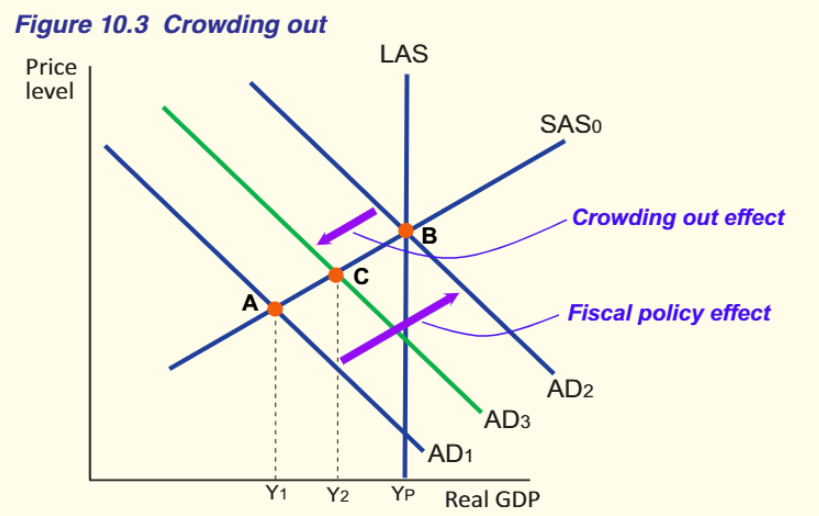
Figure 10.3 uses the AD/AS model to show the impact of crowding out. Initially the economy is at point A with real GDP below to potential GDP at Y1 (a negative output gap). The government decides to increase its spending in order to move the economy to point B. The intention is to increase aggregate demand from AD1 to AD2.
However, if crowding out occurs, then consumption and investment will fall which will reduce the expansionary impact of the higher government spending. The AD curve will only shift to AD3.
Does ‘crowding out’ occur all the time?
No, not if the economy is in a recession, because private spending is already low and unlikely to fall in response to government stimulus.
The advantage of borrowing from domestic residents is that there is no increase in the money supply and so inflation is not likely to be a problem. Also, borrowing from domestic residents means that the government is effectively borrowing from itself - this means that interest payments on the bonds will be paid back to its own citizens.
If the government sells bonds to foreign residents, then crowding out is not an issue. However, interest payments on the issued bonds will now be sent to overseas residents which is a net leakage from the economy. The government’s share of foreign debt will increase which may have implications for the government’s credit rating in offshore markets.
The third method of financing the deficit is for the government to borrow from the RBA by selling government bonds. This is referred to as ‘printing money’. There is a direct injection of new funds into the economy which increases the money supply and therefore is highly inflationary.
This method would only be appropriate if the economy was in a deep depression. The RBA has publicly stated that it will not facilitate this method because of its adverse effects on the rate of inflation.
The final method the government can use is to sell government assets.
For example, in the past the government has privatised certain government business enterprises. Examples include the Commonwealth Bank, Qantas, Telstra and Medibank Private. Selling government property such as public land and/or buildings is also an option to raise finance.
The problem with selling assets is that it is limited to what the government owns and cannot be sold a second time.
Privatising government enterprises may also have a negative impact on low income groups who may have relied on subsided government services.
Budget deficit and government debt
When the government borrows to fund its deficit, it increases the level of government debt. The total value of Australian Government Securities (AGS) on issue is known as the Government’s gross debt. In 2015, this amounted to $369 billion or 23% of GDP. By 2024, this value had increased to $904 billion or 34% of GDP.
This may sound alarming but when compared to the government debt ratios of the United States (120%), the United Kingdom (100%) and Japan (250%), Australia’s ratio seems quite modest.
The annual interest bill on the Australian Government’s debt is currently $23 billion. This is not an insignificant amount. This is more than double the amount the Commonwealth Government spends on housing. So, this does represent a sizeable opportunity cost.
If the Government had no debt, then it could allocate $23 billion more to areas such as housing, education or healthcare. The counter argument is that if the borrowing has been used to ‘grow’ the economy through higher levels of economic activity and increased spending of infrastructure, then the economy will actually benefit.
Government investment spending not only increases aggregate demand but also increases aggregate supply, causing potential GDP to increase. Investment in transport, energy networks and community facilities will last for many decades which means that future generations will benefit.
It is for this reason that governments should always borrow to fund public infrastructure rather than pay out of current taxation. This helps to share the burden of borrowing between current and future generations and thereby promote intergenerational equity.
What impact does a budget surplus have on public finances?
The surplus could be used to retire (pay off) government debt built up by past deficits, held over to fund future expenditure or returned to taxpayers, perhaps as a direct payment or as a tax cut.
A novel idea would be to ‘bank’ budget surpluses as a sovereign wealth fund (SWF). In years where Government revenue was unusually high, the surplus revenue could be invested in the fund so that earnings could be used to finance deficits. This is especially relevant for the Australian economy given that much of its income an wealth is derived from a finite supply of natural resources.
Automatic stabilisers and discretionary fiscal policy
Fiscal policy is divided into two parts:
Discretionary fiscal policy
Automatic stabilisers
Discretionary fiscal policy
Discretionary fiscal policy refers to deliberate or purposeful changes in the government’s spending decisions and/or rates of taxation.
Examples of discretionary policy would include increased spending on defence equipment, a change to the marginal rates of personal income tax or specfic changes in the excise duty on alcohol and tobacco.
The annual Budget Statement specifies all the discretionary changes in expenditure made across the various functions of government.
Automatic stabilisers refer to the changes that occur automatically to government transfer payments and tax revenue due to changes in the business cycle.
For example, if the economy contracts and real GDP falls, then automatically various welfare payments, including unemployment benefits, will automatically increase.
At the same time, as economic activity declines, revenue from both personal income tax and company tax will decrease. If we combine these effects, then whenever the economy slows or contracts, the budget balance will fall and shift towards a deficit.
Is this a good feature of fiscal policy?
Absolutely because it means that fiscal policy is automatically helping to stabilise the economy.
What if the economy expands and the level of economic activity accelerates - will there be an automatic stabilising effect?
Yes, because now government spending on transfer payments will automatically fall, while tax revenue will rise. This will cause the budget balance to automatically increase and shift towards a budget surplus. So the automatic part of fiscal policy is helping the government to ‘smooth’ the ups and downs of the business cycle.
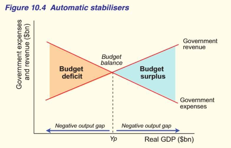
Figure 10.4 illustrates the effect of automatic stabilisers on the government’s budget balance if the economy is either below potential GDP (a negative output gap) or above potential GDP (a positive output gap). When the economy is in a negative output gap, the budget will shift to a deficit. When the economy is in a positive output gap, the budget will shift to a surplus.
Normally we would expect the budget to be balanced when the economy is at potential GDP
Expansionary fiscal policy
While automatic stabilisers are an important aspect of fiscal policy, they cannot prevent fluctuations in the business cycle. Their role is to support and complement discretionary policy in the Government’s pursuit of its economic objectives.
The Government will adopt an expansionary fiscal stance if the economy is experiencing a negative output gap, perhaps caused by the economy growing too slowly or by a negative shock that has caused the level of economic activity to fall.
An expansionary stance will mean that the Government will decrease the budget balance by either increasing its spending and/or reducing rates of tax.
This means that the Government will plan for a budget deficit.
The aim of expansionary fiscal policy is to increase or shift the aggregate expenditure function upwards in the AE model or increase the aggregate demand curve in the AD/AS model.
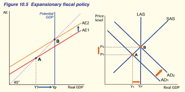
Figure 10.5 illustrates the use of expansionary fiscal policy using both the AE model and the AD/AS model. In each case, the economy is initially in equilibrium at point A where real GDP (Y1) is less than potential GDP (YP).
The unemployment rate at point A will be higher than the natural rate, while inflationary pressures are likely to be low because of a subdued economic outlook.
The government will want to stimulate spending and raise the level of economic activity in order to close the output gap and move the economy closer to potential GDP and full employment.
How can it do this?
Simply by increasing government spending (G) relative to government revenue (T), the government aims to shift the economy to point B and reduce the size of the output gap.
In each case, the increase in government spending (and/or cut taxes) will have a positive multiplier effect. However, in the AD/AS model the multiplier effect will be less than in the AE model because the price level will rise.
The AD/AS model shows that while expansionary fiscal policy will increase real GDP and reduce the unemployment rate, it will cause the price level to rise.
Whether this will increase the rate of inflation depends on the size of the negative output gap. If the economy is relatively weak, then inflationary pressures are likely to be low due to excess capacity.
Specific policy measures that the Government could use to stimulate aggregate demand could include:
increased spending in the government’s main departments such as healthcare, education and defence sectors
increasing government investment spending on infrastructure, such as transport and communications projects
increased transfer payments to low income households
reducing personal income tax to increase household consumption spending
reducing the company tax rate to stimulate business spending on resources, employment and investment.
A budget deficit will always have an expansionary effect on the level of economic activity because there is a net injection of funds into the economy, even if the budget deficit was reduced from one year to the next.
For example, suppose that the deficit in year 1 was equal to $20 billion and in year 2 the deficit had fallen to $10 billion.
What would be the impact? Assume the multiplier equals 2.5. In year 1, real GDP would increase by $50 billion (20 x 2.5) while in year 2, real GDP would increase by $25 billion. So a smaller budget deficit will still be expansionary.
Contractionary fiscal policy
The Government will adopt a contractionary fiscal stance if the economy is experiencing a positive output gap, caused by the economy growing too fast.
The positive output occurs when an economy’s actual output is greater than the potential output (meaning we are operating beyond capacity leading to increased inflation).
The level of economic activity will have risen above potential GDP causing an increase in the inflation rate due to capacity constraints.
A contractionary stance will mean that the Government will increase the budget balance by either decreasing its spending and/or increasing rates of tax.
It will plan for a budget surplus.
The aim of contractionary fiscal policy is to decrease or shift the aggregate expenditure function downwards in the AE model or decrease the aggregate demand curve in the AD/AS model.
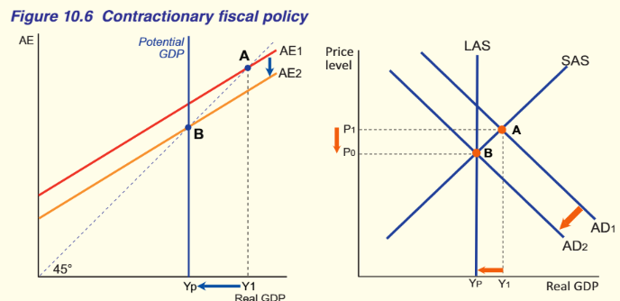
Figure 10.6 illustrates the use of contractionary fiscal policy using both the AE model and the AD/AS model. In each case, the economy is initially in equilibrium at point A where real GDP (Y1) is greater than potential GDP (YP).
The unemployment rate at point A will be lower than the natural rate, while inflationary pressures are likely to be very high because of boom like conditions.
The government will want to reduce spending and decrease the level of economic activity in order to close the output gap and move the economy closer to potential GDP and full employment.
How can it do this?
Simply by decreasing government spending (G) relative to government revenue (T), the government aims to shift the economy to point B and reduce the size of the output gap. In each case, the decrease in government spending (and/or increase in taxes) will have a negative multiplier effect.
However, in the AD/AS model the multiplier effect will again be smaller than in the AE model because the price level will fall.
Specific policy measures that the Government could use to decrease aggregate demand could include:
decreased spending in the government’s main departments such as healthcare, education and defence sectors
decreasing or postponing government investment spending on infrastructure, such as transport and communications projects
decreased transfer payments to low income households
increasing personal income tax to decrease household consumption spending
increasing the company tax rate to reduce business spending on inputs, employment and investment
Normally contractionary fiscal policy focuses on cuts in government spending rather than increases in personal income or company tax because of the political unpopularity of taxes.
But even cutting government expenditure across various government departments can be difficult since a high proportion of department spending is on wages and salaries.
A budget surplus will always have a contractionary effect because there is a net withdrawal of funds from the economy.
Even when the budget surplus is reduced from one year to the next, it will still have a contractionary effect.
A budget surplus will also always have a negative multiplier effect on the level of economic activity.
Fiscal policy and aggregate supply
Fiscal policy primarily works by affecting the aggregate demand curve - through direct changes in government expenditure and indirectly through changes in tax rates which affect consumption and investment expenditure.
In the chapter where we studied the AD/AS model, that any increase in investment expenditure, whether it be private or government - would affect not only the AD curve, but also the aggregate supply curves.
Investment increases the capital stock which adds to the productive capacity of the economy. So government investment in essential infrastructure will increase both aggregate supply curves to the right. Government spending on education is regarded as investment in human capital because it can increase the skills and productivity of labour so this is another way the government can affect the supply side of the economy.
If the government decreases the marginal rates of personal income tax, this will increase the incentive for people to work more and will therefore expand the labour force. Increases in the labour force also add to the economy’s productive capacity and will shift the AS curve to the right.
A cut in the company tax rate will increase the profitability of firms, which is a key determinant of business investment. An increase in private investment by adding to the capital stock will also shift the AS curves to the right helping to increase potential GDP.
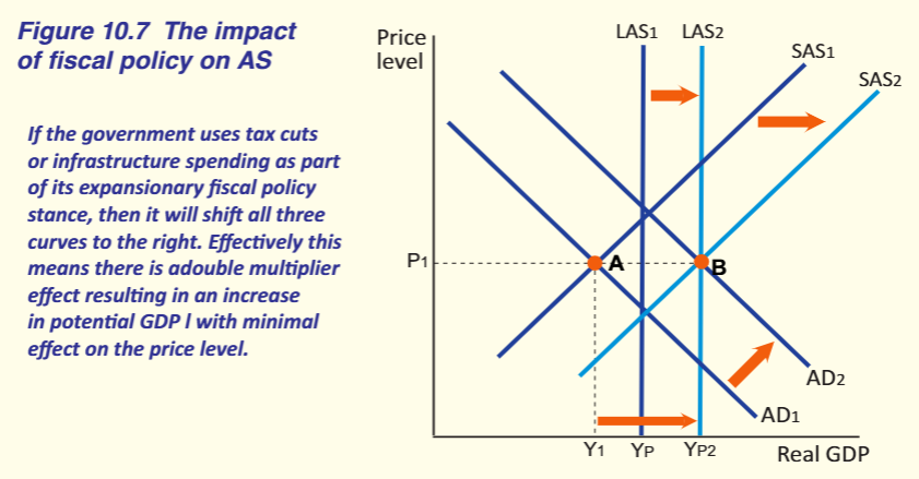
This figure illustrates this additional power of fiscal policy to affect the ‘supply side’ of the economy. The significance of this is that a decrease in tax rates (either income tax or company tax) will have a dual effect on the level of economic activity and real GDP.
There will be an initial multiplier effect from the increase in aggregate demand and then a further stimulus from the increase in aggregate supply.
All three curves in our model will shift to the right - the AD, the SAS and the LAS curve. But that’s not all - the bonus is that there will be little impact on the price level because aggregate supply has increased.
Strengths of fiscal policy
Fiscal policy has a number of advantages in helping the government to achieve its economic objectives.
Advantage 1
Fiscal policy is a very direct policy to affect aggregate demand. Revenue and spending measures announced in the Budget can be implemented relatively quickly.
For example, stimulus payments were sent to all households and firms at the start of the Covid pandemic. This represents an immediate injection of funds into the economy.
The Treasurer might announce an increase in the excise tax on a commodity from the day after the Budget, or a reduction in the marginal rates of income tax from a specific date. Consumers feel the impact of these decisions as soon as the government legislation is passed.
Advantage 2
Fiscal policy is that government spending can be targeted to specific groups or sectors of the economy. This means that the government could target low income groups for special income payments or target high income groups with higher taxes on luxury products. Many government services are means tested to ensure that the services are provided to those most in need.
Advantage 3
It is effective in times of recession. The government can open a ‘spending tap’ to increase the level of aggregate demand in order to boost employment and output. This will have an immediate multiplier effect and cushion the impact of the business cycle contraction.
During the Covid recession of 2020, the Australian government undertook massive stimulus measures to keep households and firms spending and to save jobs and businesses.
All types of government policy are faced with the problems of time lags. These lags can be split into two broad types - the inside lag and the outside lag.
The inside lag refers to the time it takes to undertake a policy action and includes the recognition, decision and implementation lags.
The outside lag refers to the time it takes for the policy to actually affect the level of economic activity. This is also known as the effect lag and it is where fiscal policy shines.
Fiscal policy has a very short effect lag because changes in both government spending and tax rates will have an immediate impact on both household consumption and business investment.
An increase in government spending will directly increase aggregate demand creating a positive multiplier effect on the level of economic activity.
An income tax cut will immediately increase workers pay-packets resulting in an increase in household consumption which will then flow on to stimulate further spending.
Other strengths of fiscal policy such as automatic stabilisers help to complement discretionary policy in ameliorating the effects of the business cycle. The positive effects fiscal policy can have an increasing aggregate supply through government investment reductions in income and company tax rates.
Weakness of fiscal policy
Fiscal policy also has a number of disadvantages which can reduce its effectiveness in its countercyclical role.
Fiscal policy has a relatively long inside lag which consists of the decision and implementation lags.
This is because discretionary changes to fiscal policy have to be debated and voted on in Parliament. This can ‘eat up’ valuable time which can delay the implementation of fiscal measures.
The fiscal policy is viewed as being relatively inflexible. The Budget is delivered once a year and while there is a mid year review, it is difficult to make wholesale changes to its spending and revenue plans.
Fiscal policy can be thought of as a ‘supertanker’ sailing in the ocean, once moving it has considerable power but if it needs to suddenly alter course or change direction, it make time considerable time to do so.
While fiscal policy is especially suited to stimulating an economy during a recession, it is less effective when trying to contract the economy.
Decreasing government spending and/or increasing tax rates during boom conditions, for example, would not be popular with the electorate.
In developing the Budget, Treasury may not be able to make large changes to the patterns of spending established from previous years.
Both social and demographic constraints need to be considered. It would be impossible, for example, to reduce spending in a boom by cutting all defence spending or slashing social security payments. Similarily it is unlikely that social security benefits could ever be increased by more than a small amount at a time, because funding larger benefits may reduce incentives for people to work.
Fiscal policy is under the control of the incumbent political party that has been elected into power. This means that fiscal policy is very likely to suffer from political bias.
The government in seeking re-election, may use fiscal policy to win favour with voters rather than address important economic and/or social issues.
The Governmnet, for example, would have an incentive to deliver an expansionary budget prior to an election in order to ‘win’ votes.
However, this may exacerbate an existing inflation problem and create a conflict with the Reserve Bank and monetary policy. This situation, in fact was played out in 2024 when the monetary policy stance was contradictionary, but the fiscal policy stance was expansionary.
Fiscal and monetary policy should be working to achieve the same objectives rather than be in conflict.
An important effect is the unintended impact on decisions taken in the private sector. The crowding out concept referred to earlier suggests that when the government runs a budget deficit it can decrease both consumption and investment spending.
This means that the impact of the increased government spending will be partly cancelled out.
There is both physical crowding out where the government competes with the private sector for limited resources and there is financial crowding out where the increased demand for funds increases interest rates.
If the economy is in a recession, then the problem of crowding out will be minimal. But if the economy is operating close to full employment and the government pursues expansionary fiscal policy, then crowding out will be significant.
Recent fiscal policy performance
Is there a simple rule that we can use to measure the effectiveness of fiscal policy over time?
We can always measure the Government’s performance in terms of achieving its policy objectives such as sustainable growth, full employment and price stability.
During 2024, the unemployment rate averaged 4%, the inflation rate was 3.5% and real GDP grew at just 1%.
Another criteria we could use is to compare the budget outcomes over an extended period of time when the economy has been through a full business cycle.
This would mean that in years when the economy was buoyant with strong growth and low unemployment, the budget would record surpluses.
While in years when the economy was weak and/or in recession, the budget would record deficits. If we summed the deficits with the surpluses over time, they should cancel out. This would also maintain a stable level of government debt.
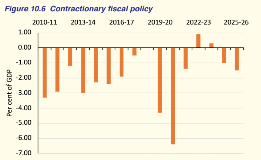
Figure 10.8 illustrates Australia’s budget balance from 2010 to 2025-2026. Of the 16 years covered in the graph, 12 years recorded a budget deficit, one year was in balance and just two years recorded a budget surplus.
If we summed the 16 years will we get a zero balance?
The answer is an empathetic no, which means that the economy’s fiscal performance has been less than optimal over this period.