Week 6: Univariate and Multivariate

Introduction to Data Preparation Pt 2

• Last week's module covered preliminary procedures for preparing a data file for analysis.

• This module focuses on procedures to complete before conducting inferential analyses.

Univariate Profiling: Getting Familiar With the Data

• Inspect univariate distributions to identify potential problems.

  • Restricted range.

  • Univariate outliers.

  • Shape of the distribution.

• Univariate profiling: becoming familiar with each variable.

Check for Restricted Range

• Restricted range: Occurs when scores do not cover the entire possible range or are concentrated in a narrow range.

• Consequences of restricted range:

  • Reduced sensitivity: Insufficient variation in scores. Difficult to distinguish between participants.

  • Distorted effects: Increased risk of Type II errors. Effects may appear smaller than they are.

  • Sample bias: Limits generalizability and external validity.

Identifying Restricted Range

• Inspect descriptive statistics (min/max values) and histograms for each variable.

Descriptive Statistics Example

• Variables: Compensation, Leadership, Work Demands, Collegiality (measured from 1 to 10).

• Observe minimum and maximum scores.

  • Compensation: Maximum score is only 5, indicating restricted range.

  • Smaller standard deviation due to less room for variability.

Histograms

• Restricted range is evident when there is a gap in the histogram where scores are expected.

• Example: Satisfaction with compensation measured from 1 to 10, but histogram stops at 5.

What To Do If You Have Variables with Restricted Range

• If due to missing data:

  • Collect more data (case substitution).

  • Estimate missing values (estimation maximization and multiple imputation).

• If you can't collect more data or estimate the missing values:

  • Conduct inferential analyses with caution.

  • Acknowledge potential impacts: higher likelihood of Type II error, suppressed effect sizes, and/or sample bias.

  • This is the main approach if working with Jamovi, as it can't perform estimation maximization or multiple imputation.

Univariate Outliers

• Extreme scores on a single variable.

• For ungrouped data: include all participants.

• For grouped data: check for outliers within each group.

• Identifying Univariate Outliers Statistically

  • Transform scores into Z scores.

  • $Z = \frac{X - \mu}{\sigma}$

  • Z-scores: standardized scores representing the number of standard deviations a data point is from the mean.

  • Sign indicates if the data point is above or below the mean.

  • Magnitude indicates how many standard deviations from the mean.

  • Example:

  • $Z = 1.50$: 1.50 standard deviations above the mean.

  • $Z = -2.30$: 2.30 standard deviations below the mean.

  • p < .001

  • $Z$ scores of $+/ - 3.29$ are considered significantly different from the mean.

Identifying Univariate Outliers Graphically

• Box plots: Depict median, 25th and 75th percentiles, and whiskers (1.5 x Interquartile Range).

• Values outside the whiskers are flagged as outliers.

What To Do If You Have Univariate Outliers

• Do Nothing: Common with large samples; analyses are often robust.

• Remove the outliers: Delete or filter out participants if the outlier is not a genuine participant.

• Windsorise the outlier: Replace the outlier with the next highest value that isn't an outlier.

• Transform the variable: Apply a formula to make the distribution more normal, squashing the tail closer to the center.

Evaluate Univariate Normality

• Assess if each variable is normally distributed.

• Ideal for sufficient variability and sensitivity.

• Check normality within each group for grouped data.

When is Non-Normality A Problem?

• Not always an issue for assumption testing; the central limit theorem applies with large sample sizes (n > 30).

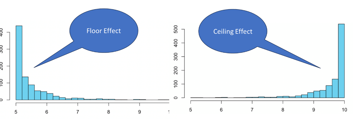
• Problematic if it impacts multivariate normality or indicates floor/ceiling effects.

  • Floor effect: A floor effect occurs when a large number of participants score at or near the lowest possible value on a measurement scale. This results in a substantial positive skew (a peak to left-hand side with a tail extending up to the right of the distribution). 

  • Ceiling effect: A ceiling effect occurs when a large number of participants score at or near the highest possible value on a measurement scale. This results in a substantial negative skew (a peak on the right-hand side with the tail extended down to the left of the distribution).

  • 

Why are Floor and Ceiling Effects a Problem?

• Reduce sensitivity of a measure.

• Lead to reduced variability, reduced power, higher risk of Type II error, and suppressed effect sizes.

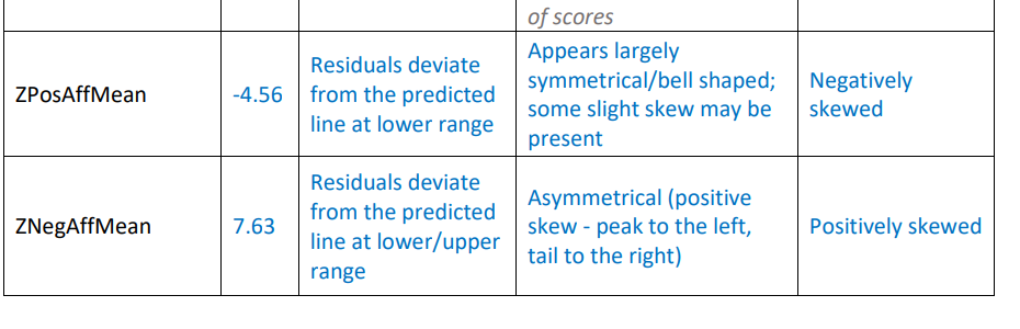
Evaluating Univariate Normality Statistically

• Use standardized skewness scores (ZSkew).

• $Z<em>{skew} = \frac{Skewness}{Standard \ Error</em>{Skewness}}$

• Score of zero: perfectly symmetrical distribution.

• Higher magnitudes: greater deviations from normality.

• Sign: indicates positive or negative skew.

• $Z$ scores greater than $+/- 3.29$ indicate significant deviation from normality (significant skew).

Evaluating Univariate Normality Graphically

• Histograms: Normal distribution appears bell-shaped and symmetrical.

• Q-Q (Quantile-Quantile) plots: Compare the distribution shape against a normal distribution; points should fall along the diagonal line.

• 

What To Do If Variables Are Not Normally Distributed

• Not necessarily a problem unless it causes issues with multivariate normality.

• Address problems with univariate normality:

  • Remove outliers.

  • Transform the variable.

• If normality cannot be fixed, consider non-parametric analyses or robust methods (e.g., bootstrapping).

Checking Univariate Outliers and Normality Within Groups

• For group data, check univariate outliers and normality within each group separately.

• Split the sample into groups using the grouping variable.

Multivariate Outliers

• Unusual combinations of scores on two or more continuous variables.

• Not always a problem, especially in large samples.

When are Multivariate Outliers a Problem?

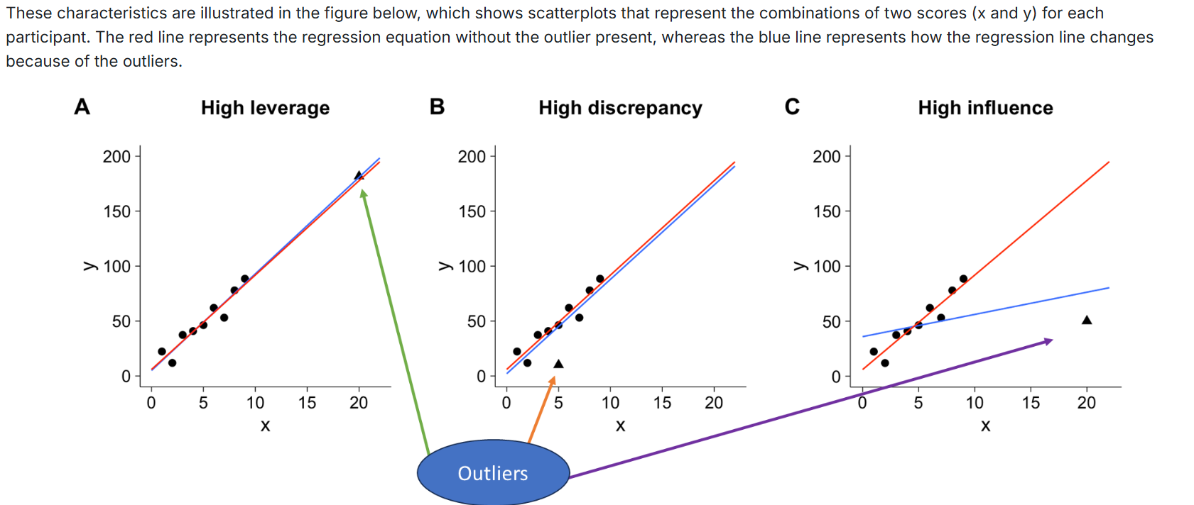
• The problem occurs when outliers have high influence.

  • Influence: Degree to which an outlier distorts the regression equation.

  • Combination of leverage (distance from other data points) and discrepancy (how far out of line the data point is from others).

  • 

Evaluating Multivariate Outliers

• If working with grouped data, evaluate outliers separately within each group.

Step 1: Identify Multivariate Outliers

• Use Mahalanobis Distance: measures the distance of each participant from the centroid, accounting for covariance.

• A significant Mahalanobis Distance indicates a multivariate outlier.

Step 2: Inspect the Outliers

• Check if the outlier is a genuine participant.

• Check for data entry errors.

• Check if they are a member of the population of interest.

• If the multivariate outlier appears genuine, evaluate their influence.

Step 3: Evaluate Influence

• Calculate Cook's Distance scores: measure of influence. Cook's \ Distance > 1.00 is a cause for concern.

• Run analyses with and without the outlier to see if the results change.

  • If the significance, effect size, magnitude, and precision of estimates change substantially, the outlier has high influence.

Step 4: Decide What to Do About Outliers

• If outliers appear genuine, but influence the results:

  • Check if scores are also univariate outliers; consider winsorizing or transforming.

  • If not univariate outliers, decide whether to remove the participant or retain them.

Assumption Testing: Multivariate Normality

• Most multivariate analyses assume multivariate normality.

  • All linear combinations of all variables are normally distributed.

• Evaluate by examining the distribution of the residuals of a model.

  • If residuals are normally distributed, multivariate normality can be assumed.

• Use Q-Q plots of residuals.

• Violations of multivariate normality impact some analyses more strongly than others.

What To Do If Multivariate Normality is Violated

• ANOVA models are robust to violations, especially with larger sample sizes; consider non-parametric alternatives if the violation is extreme.

• Analyses based on correlation can be heavily impacted.

Strategies to address problems with multivariate normality

• Remove univariate and/or multivariate outliers.

• Try fixing univariate problems using data transformations.

Other Assumptions of Multivariate Analyses

• Regression models:

  • Linearity: The relationship between the residuals and values predicted by the regression model are linear.

  • Homoscedasticity: the variability or spread of residuals is equal at all levels of the predicted values.

  • Independence: Residuals are independent.

  • Collinearity: Independent variables are not collinear.

• Factor Analysis (Exploratory Factor Analysis):

  • Sampling adequacy: The variables must be sufficiently correlated for a factor analysis.

• Between-Groups Factorial ANOVA:

  • Homogeneity of variance: The variance in the dependent variable is equal between each group.

• Repeated Measures and Mixed Factorial ANOVA:

  • Homogeneity of variance.

  • Sphericity: there is equal variance in the difference scores between each time point/measurement.

Data Transformations

• Statistical techniques used to modify the distribution of a skewed variable to make it closer to a normal distribution.

• Squashes the tail of the skewed variable back towards the rest of the data.

• Common normality transformations:

  • Square root.

  • Logarithmic.

  • Inverse.

  • Follow this order of transformations to avoid over-transformation.

  • 

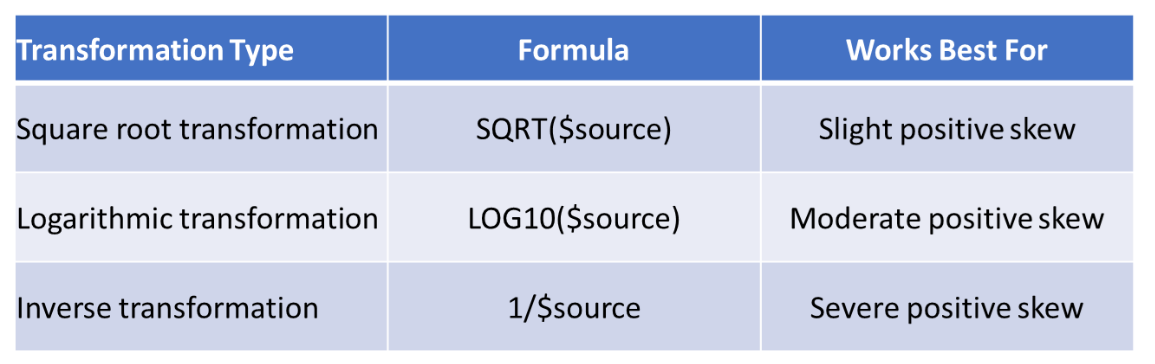
Common normality transformations Formulas in Jamovi

• Square root: SQRT($source)

• Logarithmic: LOG($source)

• Inverse: 1/$source

Formula to reflect a variable

• (f(x) = (highest
  value + 1 - $source))

• To reflect a variable, we apply the following formula: fx = (highest value + 1 - $source)

A Word on Caution on Normality Transformations

• Can be controversial.

• Transformed variables can be difficult to interpret.

• Transformations are not necessary if analyses are robust to violations of normality.

• Transforming won't always fix problems with multivariate assumptions.

Final Stages

• Prepare data and conduct inferential analyses to test hypotheses