L29 - Electrical Circuits (Electrical Current)
Classification and Physical Distinction: Insulators vs. Dielectric Materials

Fundamental Distinction Between Electrical Insulators and Dielectrics:
All dielectric materials are electrical insulators, but not all insulators are dielectric materials.
An insulator is defined strictly by the absence of free charge carriers within its bulk structure. Consequently, it strongly opposes and resists any flow of external electrical charge attempted through the material, exhibiting high electrical resistance and high resistivity.
A dielectric material is an insulator that possesses the specific property of being polarizable when placed within an external electric field ().
Polarization occurs either through molecular deformation (inducing dipole moments in nonpolar structures) or through the spatial reorientation of native permanent dipoles along the direction of the applied field.
The creation and alignment of these internal dipoles generate an internal induced electric field and enable dielectrics to store electrical potential energy.
Certain materials, such as specific formulations of ceramics, act as insulators by preventing charge flow, yet exhibit negligible or zero polarization in external electric fields, meaning they do not act as dielectrics.
Non-Equivalence of Polarizability and Electrical Resistivity:
Polarizability () is the proportionality constant relating the induced dipole moment () to the local electric field ().
Resistivity () quantifies the inherent opposition of a material to the conduction of electrical current.
There is no direct, proportional, or monotonic relationship between polarizability and resistivity:
Glass vs. Distilled Water Example:
The relative permittivity (dielectric constant, ) of glass is approximately .
The relative permittivity of distilled water is approximately .
Water exhibits a significantly higher polarizability () than glass under identical external electric fields.
Glass possesses an extraordinarily higher resistivity () to charge flow than distilled water.
A higher polarizability does not imply higher electrical resistivity, nor does it imply lower resistivity.
While all dielectrics exhibit much greater resistivity than conductors, variations in polarizability among dielectrics do not correlate directly with their comparative resistance to current.
Electrostatics of Dielectrics in Capacitors

Parallel Plate Capacitor in Vacuum:
Consider two conducting plates of finite area () separated by a distance (), carrying equal and opposite total charges ( and ).
The surface charge density of the conducting plates is defined by:
Assuming the plate dimensions are large relative to the separation distance (), fringing field effects at the plate edges can be neglected.
The electric field lines point strictly from the positive plate toward the negative plate.
The uniform electric field magnitude in vacuum () between the plates is given by: where is the electric permittivity of free space (, or order of magnitude ).
Influence of a Dielectric Medium on Capacitance and Field:
When the gap between the plates is filled with a dielectric medium, the absolute permittivity becomes , where is the relative permittivity (also designated as the dielectric constant, ).
Because for all physical dielectric media, the net electric field inside the capacitor is reduced relative to vacuum:
Capacitance () is defined as the charge stored per unit of electrical potential difference ():
For a parallel plate geometry filled with a dielectric:
The presence of a dielectric increases the capacitance by a factor of , allowing more charge and energy to be stored at a given potential difference.
Microscopic Polarization Mechanisms:
Polarization by Deformation: Occurs in nonpolar atoms and molecules (such as helium gas). The external electric field shifts the electron cloud relative to the positive nucleus, inducing an electric dipole moment. This mechanism typically results in lower polarizability.
Polarization by Orientation: Occurs in molecules possessing native, permanent dipole moments (such as distilled water). In the absence of an external field, thermal motion randomizes the orientation of the dipoles, resulting in zero net macroscopic dipole moment.
Thermal Agitation: In orientation polarization, elevated temperature increases the kinetic/thermal energy of the molecules, randomizing orientations and reducing the net average polarizability ().
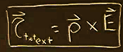
Torque on Native Dipoles: An external electric field exerts an electrostatic force on the opposite charges of each dipole, producing a net torque () about its center of mass:
By convention, the electric dipole moment vector () points from the negative charge to the positive charge. The torque acts to align parallel to the applied electric field ().
Superposition and Surface Bound Charge:
Each aligned microscopic dipole produces its own local field directed from its positive pole to its negative pole, which points in the opposite direction to the applied external field.
By the principle of superposition, the internal microscopic dipole fields partially cancel the applied field throughout the dielectric volume.
In the interior bulk of a uniformly polarized dielectric, adjacent positive and negative charges of neighboring dipoles cancel out, leaving the bulk interior electrically neutral.
At the physical boundaries near the conducting plates, cancellation cannot occur:
A bound polarization surface charge (, or ) forms on the dielectric surface adjacent to the positive conducting plate.
A bound polarization surface charge (, or ) forms on the dielectric surface adjacent to the negative conducting plate.
These bound charges behave like a secondary, opposing parallel plate configuration separated by approximately the same distance ().
Analytical Derivation: Polarizability, Electric Susceptibility, and Relative Permittivity

Net Electric Field in Terms of Polarization Charge:
Expressing the electric fields purely in magnitude, the net electric field () inside the dielectric is the difference between the field generated by the free charges on the plates () and the opposing field generated by the induced bound polarization surface charges (): where is the free surface charge density on the plates (), and is the induced polarization surface charge density ().
Relation of Induced Charge Density to Microscopic Dipoles:

Consider an infinitesimal volume element at the dielectric boundary of cross-sectional area and depth equal to the average dipole separation distance .
Let denote the volumetric number density of dipoles (number of dipoles per unit volume, with units of ).
The infinitesimal bound polarization charge () enclosed within this volume is:
Since the microscopic dipole moment magnitude is :
The polarization surface charge density () is therefore:
Incorporation of Polarizability and Electric Susceptibility:

The average dipole moment is linearly related to the local electric field through the polarizability ():
Substituting this relation yields the bound surface charge density:
The product of the volumetric number density of dipoles and the atomic/molecular polarizability is defined as the electric susceptibility ():
Derivation of Relative Permittivity ():
Substitute back into the net electric field expression:
Rearrange terms to isolate the free charge field term ():
Solving for the net electric field ():
Comparing this result with the definition of the net field in a dielectric () establishes the relationship:
Physical Orders of Magnitude:
Polarizability () typically has an extremely small magnitude on the order of .
Vacuum permittivity () is of the order .
The volumetric dipole density () is extraordinarily large (billions of molecules per cubic millimeter, scaling with Avogadro\u0027s scale densities).
Consequently, the dimensionless term can vary substantially depending on the substance:
For gases or dilute media: .
For liquid water: .
Self-Consistency Approximation Caveat: This derivation equates the polarizing field acting on the individual molecules directly to the net field (). Rigorously, the local field acting on a molecule includes the external field plus the fields of all other surrounding dipoles (), which creates a recursive self-consistent formulation. Setting the local field equal to the macroscopic field provides an accurate, mathematically tractable first-order model.
Practical Application: Microwave Heating via Dipole Rotation
Working Principle of a Microwave Oven:
Biological tissue and most foods are predominantly composed of liquid water, which consists of permanent, native electric dipoles.
A microwave oven exposes food to an alternating electromagnetic field oscillating in the gigahertz () frequency band (billions of polarity reversals per second).
At any fixed location inside the cavity, the electric field vector reverses direction billions of times per second ().
The permanent water dipoles experience a rapid, alternating torque attempting to reorient them into alignment with the oscillating field.
Because the field oscillates at such high frequencies, rapid rotation causes continuous inelastic collisions with neighboring molecules.
These collisions convert rotational potential and kinetic energy into randomized thermal kinetic energy, raising the macroscopic temperature of the food.
Although higher temperatures marginally decrease the orientation polarizability (), the coupling remains sufficient to heat the food.
Microwave radiation at these wavelengths penetrates deeply into the food volume without severe immediate surface attenuation, producing relatively isotropic, volumetric heating throughout water-rich regions, unlike conventional conductive heating.
Microscopic Dynamics of Charge Carriers in Conductors

Transition from Electrostatics to Electrodynamics:
In electrostatics, free charges redistribute until the internal electric field inside an isolated conductor reaches zero ().
In electrodynamics, an electric field is continuously maintained within the conductor (), driving a sustained non-equilibrium motion of charge carriers known as electrical current.
Charge Carrier Convention:
The physical charge carriers in metallic conductors are negatively charged free electrons ().
Historically, current was postulated to be the flow of positive charge carriers.
By convention, current is analyzed as the apparent motion of positive charges () moving along the direction of the electric field vector, while retaining the true physical inertial mass of the electron (, or order of magnitude ).
Thermal Motion and the Fermi Velocity:
In a metallic crystalline lattice (e.g., copper), valence electrons dissociate from individual atomic nuclei to form a delocalized Fermi gas of free electrons.
At temperatures above absolute zero (), these electrons possess significant kinetic energy known as the Fermi energy (): where is the Fermi velocity.
For copper at room temperature (), the Fermi velocity is approximately:
In the absence of collisions, an electron moving at would traverse the distance from Milan to Sicily in approximately one second.
In an isolated conductor without an external field, electrons undergo frequent collisions with the vibrating copper lattice ions.
Because thermal velocity vectors are distributed isotropically in random directions, the spatial and ensemble average velocity () of the billions of free electrons is strictly zero:
Consequently, there is no net displacement of charge, no net current, and no magnetic field generated by thermal motion alone.
Derivation of Drift Velocity and the Drude Model Mechanism

Acceleration Under an Internal Electric Field:
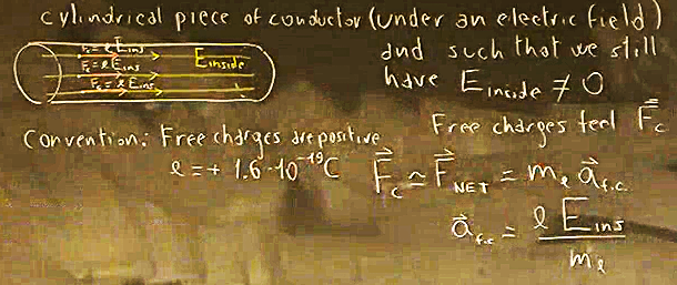
When an electric field () is sustained inside a cylindrical conductor, each mobile carrier experiences an electrostatic Coulomb force:
Gravitational forces between charges and external gravitational forces are negligible compared to the Coulomb force ().
According to Newton’s second law, the continuous acceleration () of a charge carrier between collisions is:
In a theoretical superconductor lacking scattering mechanisms, carriers would accelerate indefinitely under this constant force.
Relaxation Time and Inelastic Collisions:

In standard conductors, electrons undergo frequent inelastic collisions with lattice ions, transferring acquired kinetic energy to the lattice as thermal energy.
Let denote the mean free time (average relaxation time between successive collisions).
The instantaneous velocity () of a carrier immediately prior to its -th collision is given by its velocity immediately following the -th collision () plus the velocity increment gained from acceleration over time :
The post-collision velocity () represents the randomized thermal velocity ().
Drift Velocity () Formulation:
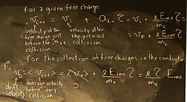
Taking the ensemble average over the vast population of free charges:
Since the thermal velocities average to zero (), the net average directed velocity—defined as the drift velocity ()—is:
Apparent Physical Paradox: In classical mechanics, an applied force produces an acceleration (). However, macroscopic charge transport displays a velocity that is directly proportional to the applied force/field (). This occurs because periodic collisions act as a drag force, repeatedly resetting the acceleration cycle and resulting in a terminal average drift velocity.
Temperature Dependence of : Increasing temperature intensifies lattice vibrations, increasing collision frequency and shortening . Thus, higher temperatures reduce drift velocity for a given field.
Order of Magnitude in Copper:

Evaluating copper at under an electric field of , with and :
Disparity of Scales: While individual electrons move violently in random trajectories at the Fermi speed of , the entire ensemble slowly drifts collectively down the wire at a rate of only .
Macroscopic and Microscopic Current: Current Density and Flux

Definition of Electric Current ():
Electric current () is a scalar quantity defined as the net quantity of charge () passing through a specified cross-sectional area per unit time ():
The SI base unit of electric current is the Ampere (), equivalent to Coulombs per second ().
Analogy to Fluid Dynamics (Volume Flow Rate vs. Charge Flow Rate):
In fluid mechanics, the volumetric flow rate () through a surface is given by the flux of velocity through the area vector: , having units of .
To convert a volumetric flow rate into an electrical charge flow rate, the volume must be multiplied by the volumetric free charge density (), which has units of :
Microscopic Current Density Vector ():
Let be the number density of free conduction charges per unit volume ().
The total mobile charge density is given by the product of the carrier density and elementary charge: .
The current density vector () is defined as the product of the charge density and the drift velocity vector ():
Units of :
General Flux Formulation of Current:
Consider a flat surface element of area characterized by an outward normal area vector .
If the current density (aligned with and ) forms an arbitrary angle with respect to the surface normal vector , current is computed via the vector dot product:
When the internal field and current density are perpendicular to the cross-sectional plane (, ), the relationship simplifies directly to:
Questions and Discussion
Ash\u0027s Inquiry on Polarizability vs. Insulating Resistance:
Prompt: Can the polarizability of a material be directly correlated to its ability to insulate or resist the flow of electric current?
Response: There is no direct or simple mathematical relationship between polarizability and resistance/resistivity. For example, water has a relative permittivity around and polarizes far more easily than glass (relative permittivity ), yet glass exhibits vastly higher electrical resistivity against charge flow than distilled water. Dielectric behavior characterizes internal bound dipole formation and energy storage, whereas insulation characterizes the absence of free carriers and opposition to charge flow.
Superposition and Sign Conventions in Capacitor Fields:
Prompt: In determining the net electric field (), why are negative signs used, and why is the denominator simply for the dielectric region?
Response: The calculation is evaluated in scalar magnitude. The original free charges on the conducting plates create a field pointing from positive to negative. The polarized dipoles align such that their negative ends face the positive plate and their positive ends face the negative plate, creating an induced surface charge that generates an internal field pointing in the directly opposite direction. Because the bulk interior is neutral due to pairwise cancellations, the space can be treated geometrically like vacuum bounded by two opposing sets of surface charge sheets ( and ), both governed by .
Layman Interpretation of Permittivity as Allowing Flow:
Prompt: Can permittivity be conceptualized simply as the degree to which a material restricts or allows electricity to flow through it?
Response: No. Electric fields do not "flow." Allowing charge to flow is the property of electrical conductivity (or inversely, resistance and resistivity). Permittivity describes how a dielectric medium polarizes and opposes the applied electric field internally through the formation of opposing dipoles. Confusing permittivity with current transmission conflates electrostatics/polarization with electrodynamic charge conduction.
Current Flow During Polarization:
Prompt: Does an electric current flow forward to establish the polarization inside a dielectric?
Response: In a static dielectric setting, there is no continuous electric current flowing through the material. Polarization involves only the microscopic displacement of bound charges (deformation of electron clouds or local rotation of dipoles), not the long-range transport of free charges.