Chapter 3: Describing, Exploring, and Comparing Data

Section 3.1 Measures of Center

A measure of center is a value at the center or middle of a data set

Different Measures of Centers

The Arithmetic mean of a set of values is the measure of center found by adding the values and dividing the total by the number of values
- Is pretty much the average of a set of values
The Median of a data set is the measure of center that is the middle value when the original data values are arranged in order of increase (or decreasing) magnitude
- If you have an even number of data points (leaving two values that share the middle), add the two numbers together an divide by two to get the median
The Mode of a data set, often denoted by M, is the value that occurs most frequently
- In the case that there is no numbers that are repeated, there is NO mode
- Sometimes, the mode can include two numbers
  - In this case, the set is called bimodal
- Three+ datapoints can be repeated the same number of times
  - In this case, the set is called multimodal, but typically you just put no mode
The midrange is the measure of center that is the value midway between the highest and lowest values in the original data set
- Add the two end values together and divide the sum by two to get the midrange

Example 1

When investigating times required for drive-through service, the following results (in seconds) were obtained. Find the mean, median, mode, and midrange for reach of the two samples. Then compare the two sets of data.

McDonald’s: 287, 128, 92, 267, 176, 240, 192, 118, 153, 254, 193, 136

Jack in the Box: 190, 229, 74, 377, 300, 481, 428, 255, 328, 270, 109, 109

McDonald’s

Mean = $\frac{2236}{12}$ ≈ 186.3

Mode = No mode

Median = $\frac{176+192}{2}=184$

Midrange = $\frac{92+287}{2}=189.5$

Jack in the Box

Mean = 262.5

Mode = 109

Median = 262.5

Midrange = 277.5

Section 3.2 Measures of Variation

The range of a set of data is the difference between the highest value and the lowest value

Range = (highest value - lowest value)

The standard deviation of a set of sample values is a measure of the variation of values about the mean
- Gives an idea of approximately how far many of the values are away from the center or mean value
- If you calculate the variance, you need to take the square root of the number to get the standard deviation
The variance of a set of values is a measure of variation equal to the square of the standard deviation
- If you calculate the standard deviation, you need to square that number to get the variance

Example

When investigating the times required for drive-through service, the following results (in seconds) were obtained. Find the range variance, and standard deviation for each sample, and then compare the two sets of results.

McDonald’s: 287, 128, 92, 267, 176, 240, 192, 118, 153, 254, 193, 136

Jack in the Box: 190, 229, 74, 377, 300, 481, 428, 255, 328, 270, 109, 109

Have the data entered into the calculator to find the range, standard deviation, and variance
- Stat → Edit → Fill in the Rows
- Stat → Calculate → 1-Var Stats → Enter
- Sx = Standard Deviation

ANSWERS

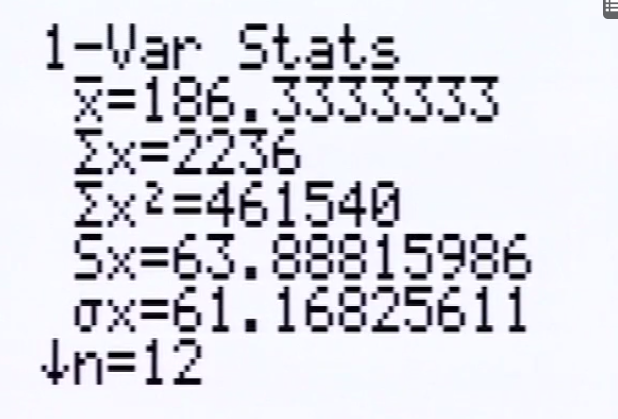
Standard Deviation (McDonald’s) = S ≈ 63.9
Variation (McDonald’s) = S² ≈ 4,083.21
Range (McDonald’s) = 195

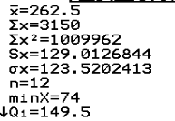
Standard Deviation (Jack in the Box) = S ≈ 129.0127
Variation (Jack in the Box) = S² ≈ 16,641
Range (Jack in the Box) = 407

Example 2

The given frequency distribution describes the speeds of drivers ticketed by the Town of Poughkeepsie police. These drivers were traveling through a 30 mi/h speed zone on Creek Road. How does the mean compare to the posted speed limit of 30 mi/h?

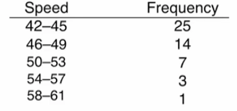
To use the calculator to find the standard deviation of a frequency distribution, we need a mid-point of each (speed) class
- ex: In row 1, the midpoint of the first class (42-45) is 43.5

Have the data entered into the calculator to find the range, standard deviation, and variance
- Stat → Edit → Fill in the Rows (and columns: one for speed, one for the frequency)
- Stat → Calculate → 1-Var Stats L₃, L₄ → Enter
- Sx = Standard Deviation

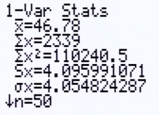
ANSWERS

S ≈ 4.096 ≈ 4.1
Variance ≈ 16.81
Range = 16

Range Rule of Thumb

To roughly estimate the standard deviation, use

s ≈ $\frac{range}{4}$

The approximation that comes from the Range Rule of Thumb is accurate when the error of it is LESS THAN 1.7 cm
Significantly low values are $\mu-2\sigma$ or lower
Significantly high values are $\mu+2\sigma$ or higher
Values not significant: Between $\left(\mu-2\sigma\right)$ and $\left(\mu+2\sigma\right)$
- μ = population mean
- σ = population standard deviation

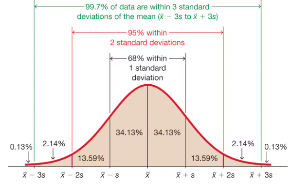
Empirical Rule for Bell-Shaped Distribution

About 68% of all scores fall within 1 standard deviation of the mean
About 95% of all values fall within standard deviations of the mean
About 99.7% of all values fall within standard deviations of the mean.
Only if the data on the graph looks like a round, semicircular, mound/bell

Example 3

Heights of women have a bell-shaped distribution with a mean of 63.6 in. and a standard deviation of 2.5 in. Using the empirical rule, what is the approximate percentage of women between 56.1 in. and 71.1 in.?

Since the problem says to use the empirical rule, that means that we have to add and subtract standard deviations from the mean
- Mean = 63.6 in.
- Standard Deviation = 2.5 in.
- 63.6 + 2.5 = 66.1
  - Not close enough to 71.1 yet
- 3x Stand. Dev. = 3(2.5) = 7.5
- 63.6 (mean) - 7.5 in. = 56.1 in.
- 63.6 + 7.5 in. = 71.1 in.
- 3 Standard Deviations from the mean is 71.1 in. AND 56.1 in.
- 99.7% of all women’s height are between 71.1 in. AND 56.1 in.

Mean Absolute Deviation (MAD)

Mean absolute deviation = $\frac{\Sigma\left|x-\overline{x}\right|}{n}$
- Step 1: Get the mean absolute deviation of each sample using this equation: $MAD=\frac{\left|a-b\right|}{2}$
- Step 2: Add all of the mean absolute deviation from each possible sample and divide by the number of samples there are

Coefficient of Variation

When comparing variation in samples or populations with very different means, it is better to use the coefficient of variation
The Coefficient of Variation (or CV) for a set of nonnegative sample or population data, expressed as a percent, describes the standard deviation relative to the mean
- Sample: $CV=\frac{s}{\overline{x}}\cdot100$
- Population: $CV=\frac{\sigma}{\mu}\cdot100$
  - μ = population mean
  - σ = population standard deviation

Section 3.3 Measures of Relative Standing and Boxplots

Relative Standing - measures that allow us to compare different data values; sometimes values in the same data set or different data values in different populations
- Example: Differences in height between husband and wife; AND differences in how tall they are compared to their respective genders
  - One way to compare the differences in how, respective to their genders, is to find the Z-Score

Z score (or standard score or standardized value) is the number of standard deviations that a given value of x is above or below the mean
- Below are the following equations:
  - Sample: $z=\frac{x-\overline{x}}{s}$
  - Population: $z=\frac{x-\mu}{\sigma}$

Notes:

s = sample standard deviation
$\overline{x}$ = sample mean
x = score
$\mu$ = population mean
$\sigma$ = population standard deviation

Z-Score Example 1

IQ Scores (Assume that the bullet points are the population parameters):

Mean = 100
St. Dev = 15

x = 160 IQ: $z=\frac{160-100}{15}$ = 4.00

What does the “4.00” mean?

The score (x) of 160 is exactly 4.00 standard deviations over the mean
- The z-score is telling you how many scores you are away from the mean
  - Positive z-score means you’re ABOVE the mean
  - Negative z-score means you’ve BELOW the mean

Typically CALCULATING z-scores isn’t the ultimate objective
One use of z-scores would be to distinguish between scores that we consider to be ordinary and unusual
- Ordinary z-scores:
  - $-2\le z\le2$
- Unusual z-scores:
  - $z<-2$
  - $z>2$
By the logic above, the IQ score from “Z-score Example 1” would be unusual because it is MORE than 2 standard deviations above what would be considered ordinary

Percentiles

99 values that partition data into 100 parts
- Example: P₂₅ (25^th percentile) is the values that separates the lowest 25% from the highest 75%
Percentile of Value x =

Percentiles Example 1

Find percentile of 72 using a data set of Female Pulse Rates:

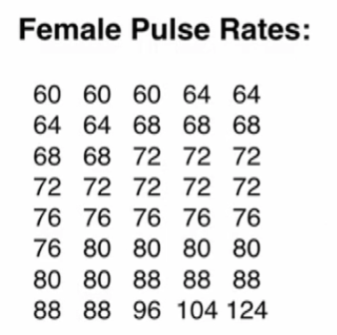
note: when working with percentiles, the list MUST be ordered (in the example, it is sorted from least to greatest)

First, ask what are the numbers less than 72.
Whatever the number is, plug it into the percentile formula

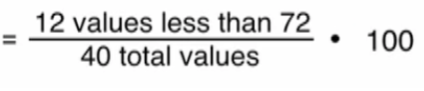
$\frac{12}{40}\cdot100=$ 30
30^th Percentile

This example shows us how to take a number from a data set and find out what it’s equivalent percentile value is

Percentiles Example 2

Given a particular data set, what is the value of the 25^th percentile?

Find P₂₅: Use flowchart from textbook

L = locator (position)
n = number of values
k = percentile

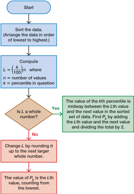
$L=\frac{k}{100}\cdot n=\frac{25}{100}\cdot40=10$

k represents the 25^th percentile
n represents the number of values (40)
The final answer is 10, which tells you the location of the 25^th percentile.
- Disclaimer: 10 is NOT the 25^th percentile by itself, it’s the location of where you could find it

By referring to the flowchart, if L turns out to be a whole number (such as 10), you go to that score and the next higher score, you have to add them together and divide by 2
- So, putting it into practice, get the 10^th number from the “Female Pulse Rates” chart (68) and add the number that is above it (the 11^th number, which is 68), and divide by 2

P₂₅ = 68

Quartiles

Q₁ = P₂₅

Q₂ = P₅₀

Q₃ = P₇₅

5-Number Summary:

Minimum (Lowest score)
First quartile Q₁
Second Quartile Q₂
Third Quartile Q₃
Maximum (Highest score)

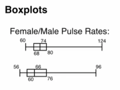
5-Number Summaries are good at forming Boxplots

Boxplots

Modified Boxplots

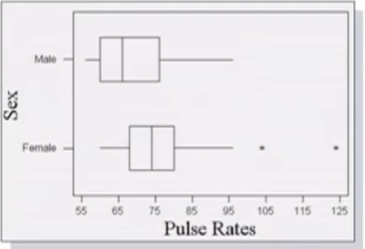
More difficult to construct than ordinary (skeletal) boxplots because they involve an interquartile range, finding the difference between the third quartile and the first quartile, multiplying that by 1.5, and more
Boxplots ISOLATE potential outliers (the dots that you see on the example boxplot, above)

Summary

Comparing Data

z Scores
Percentiles
Quartiles
5-No. Summ.
Boxplots