Chapter 8: Pure Competition in Long Run
The Long Run in Pure Competition (LO1)
In the long run, firms can adjust capacity by expanding or contracting; firms may enter or exit the industry.
Key idea: long-run adjustments involve changes in the number of firms and the scale of operations, not just output levels.
Profit Maximization in the Long Run (LO2)
In the long run, entry and exit are easy and are the primary adjustments assumed.
All firms are assumed to have identical costs (constant-cost industry).
Constant-cost industry: entry and exit do not affect resource prices; the long-run supply curve is determined by scaled-up or scaled-down industry output without shifting input prices.
Implication: firms earn zero economic profit in long-run equilibrium (normal profit) due to free entry and exit.
Long-Run Equilibrium (LO3)
Entry eliminates profits: as profits appear, new firms enter; industry supply increases; market price falls until profits are eliminated.
Exit eliminates losses: if firms incur losses, some exit; industry supply decreases; market price rises until losses are eliminated.
In long-run equilibrium under pure competition, price adjustments ensure that profits are zero (normal profit).
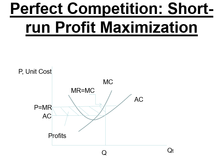
Short-run Profit Maximization in Pure Competition
In the short run, profit maximization occurs where price equals marginal revenue: .
In perfect competition, price also equals marginal cost at the profit-maximizing output: .
Output level is where ??? (intersection of MC with MR/price) yields the quantity that maximizes profit given fixed costs.
The firm’s profit equals revenue minus total cost, with total cost composed of fixed costs and variable costs.
Short-run graphs typically show the AC, ATC, MC curves and the demand/price line; profits occur when price is above average total cost, losses occur when price is below average total cost.
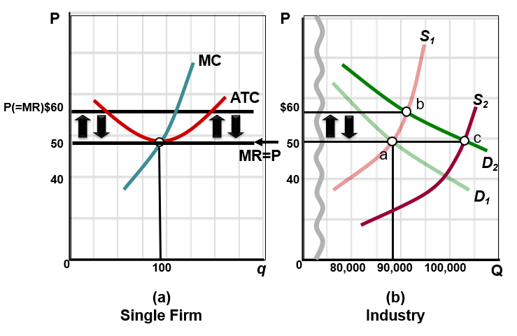
These graphs show temporary profits and the re-establishment of long-run equilibrium in (a) a representative firm and (b) the industry. A favorable shift in demand (D1 to D2) will upset the original industry equilibrium and produce economic profits (from Pt. a to b). As a result, those profits will entice new firms to enter the industry, increasing supply (S1 to S2) and lowering product price until economic profits are once again zero (Pt. b to c). In other words, an increase in demand temporarily raises price. Higher prices draw in new competitors. Increased supply returns price to equilibrium.
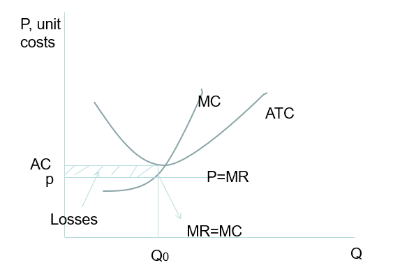
Pure Competition: SR Losses (short-run losses)
When the price is below average total cost but above average variable cost, firms incur losses in the short run.
The short-run optimal output is where MR = MC, but profits may be negative (losses).
Output quantity is denoted by Qo (short-run quantity where MR = MC).
Exit and Long-Run Adjustment (LO3)
If firms anticipate losses in the short run, some exit; this reduces industry supply and raises price toward the minimum ATC.
Long-run entry/exit drives profits to zero; the price stabilizes at the level where P = MR = MC = ATC (minimum).
The long-run impact can be depicted by shifts in the supply curve as firms enter or exit.
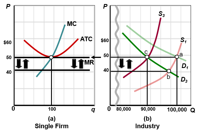
Temporary losses and the re-establishment of long-run equilibrium in (a) a representative firm and (b) the industry. A decrease in demand temporarily lowers price (from Pt. a to b). Lower prices drive away some competitors and the decrease in supply returns price to equilibrium (from Pt. b to c).
Long-Run Supply (LO4)
There are three possible industry cost structures that determine the shape of the long-run supply curve:
Constant-cost industry (1st scenario)
Increasing-cost industry (2nd scenario)
Decreasing-cost industry (3rd scenario)
The long-run supply decision depends on how LR average total cost (LRATC) responds to industry expansion.
LO4 highlights three graphs (slides 10–12): constant-cost, increasing-cost, and decreasing-cost industry supply responses.
In this first scenario, the constant-cost industry, the number of firms entering or leaving the industry do not affect costs.
In this second scenario, entry or exit of firms does affect costs. When firms enter the industry, input costs will increase as firms enter the industry and input costs will fall as firms exit the industry. The long-run supply curve is upsloping. In the decreasing cost industry, as the number of firms increase (AC decreases) or decrease (AC increases) due to entry or exit, the industry costs change inversely. If demand for their product falls, firms will leave the industry causing input costs to rise. If demand for their product increases, firms will enter the industry causing input costs to fall. The long-run supply curve is downsloping.
An example is the personal computer industry, in which the supply of personal computers increases by more than demand, causing the price of personal computers to decline. This decline in price is because the component producers (the makers of RAM, or the CPU, etc) can achieve economies of scale
Long-Run Supply: Constant-Cost Industry (LO4)
In a constant-cost industry, entry and exit do not affect LRATC; resource prices remain constant.
The long-run supply curve is perfectly elastic (horizontal) at the price that equals minimum LRATC.
Graph features (conceptual): a horizontal LR supply curve at the market price where firms earn zero economic profit; quantity supplied adjusts with demand, but price remains unchanged.
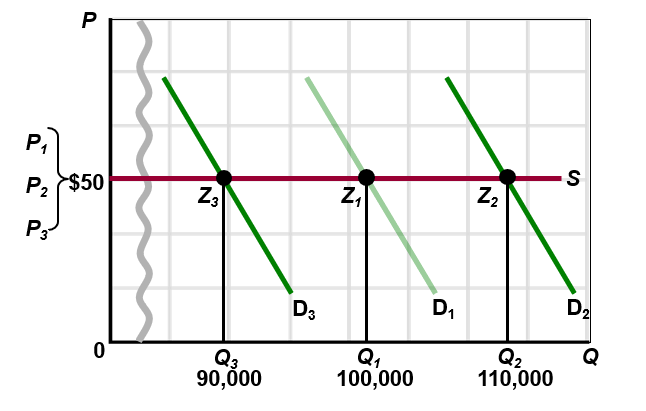
In a constant-cost industry, entry and exit of firms does not affect resource prices and therefore does not affect per-unit costs. So an increase in demand raises output but not price. Similarly, a decrease in demand reduces output but not price. Thus, the long-run supply curve is horizontal.
This happens because the new firms demand for the resources of a constant-cost industry is relatively small compared to the total demand for these resources. One example of a constant-cost industry is the cucumber (farming) industry.
Long-Run Supply: Increasing-Cost Industry (LO4)
In most real-world industries, LRATC increases with industry expansion due to rising resource input costs or bottlenecks.
As demand increases and more firms enter, prices of inputs rise, shifting LRATC upward.
The long-run supply curve slopes upward: higher prices are required to attract additional capacity.
Graph features (conceptual): LRATC rises with output, LR supply is upward-sloping in the long run.
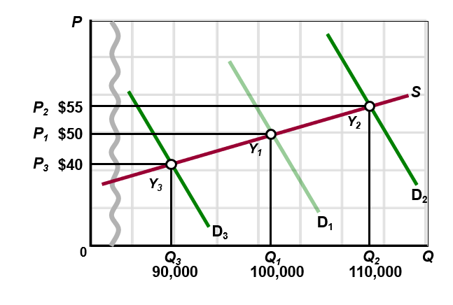
The long-run supply curve for an increasing-cost industry is upsloping. In an increasing-cost industry, the entry of new firms in response to an increase in demand (D3 to D1 to D2) will bid up resource prices and thereby increase unit costs(AC). As a result, an increased industry output (Q3 to Q1 to Q2) will be forthcoming only at higher prices ($55>$50 > $45). The long-run industry supply curve (S) therefore slopes upward through points Y3, Y1, and Y2.
Long-Run Supply: Decreasing-Cost Industry (LO4)
In a decreasing-cost industry, LRATC decreases as industry size grows, often due to economies of scale, improved efficiencies, or input price effects from larger scale.
As demand expands and more firms enter, costs per unit fall, which can shift the long-run supply curve downward.
Graph features (conceptual): LRATC falls with output, LR supply is downward-sloping in the long run.
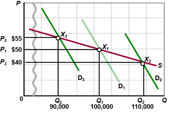
The long-run supply curve for a decreasing-cost industry is downs-loping. In a decreasing-cost industry, the entry of new firms in response to an increase in demand (D3 to D1 to D2) will lead to decreased input prices and, consequently, decreased unit costs. As a result, an increase in industry output (Q3 to Q1 to Q2) will be accompanied by lower prices ($55 > $50 > $45). The long-run industry supply curve (S) therefore slopes downward through points X3, X1, and X2.
Pure Competition and Efficiency (LO5)
In the long run, pure competition drives efficiency, with two key forms:
Productive efficiency: producing at the minimum possible average total cost, i.e., .
Allocative efficiency: producing where price equals marginal cost, i.e., .
At the long-run equilibrium in a purely competitive market, we typically have , yielding normal profit.
This state yields maximal social welfare, reflected in consumer and producer surpluses under efficient allocation.
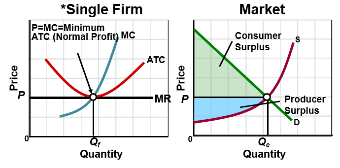
Productive Efficiency: Price=minimum ATC
Allocative Efficiency: Price=MC
Pure competition achieves both efficiencies in its long-run equilibrium. This is important because it indicates the firm is using the most efficient technology, charging the lowest price, and producing the greatest output consistent with its costs. The firm is using society’s scarce resources in accordance with consumer preferences. The sum of consumer surplus(max. price consumers willing to pay – market price) (green area) and producer surplus (market price - min. price producers are willing to produce) (blue area) is maximized.