Machine Learning

Machine Learning: how to acquire a model from data / experience

• learning parameters

  • probabilities

• learning structure

  • BN graphs

• learning hidden concepts

  • clustering

  • neural networks

Naive Bayes

Classification

• given inputs x, predict labels (classes) y

• ex. medical diagnosis

  • input: symptoms

  • classes: diseases

• ex. automatic essay grade

  • input: document

  • classes: grades

Model-Based Classification

• learn by building a model where both output label and input features are random variables

• query for the distribution of the label conditioned on the features

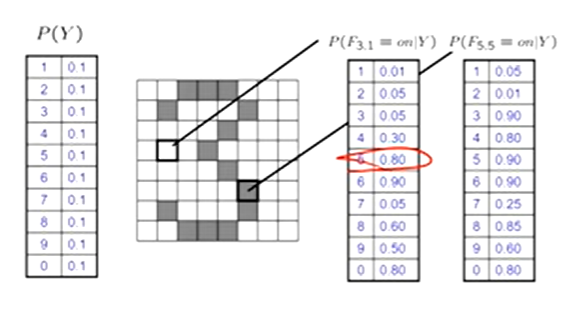
Naive Bayes for Digits

• Naive Bayes: assume all features are independent effects of the label

• Simple digit recognition version:

  • one feature (variable) F_ij for each grid position <i, j>

  • features values are on / off, based on whether intensity is more or less than 0.5

  • each input maps to a feature vector

    • ex. 1 → (F₀₀ = 0, F₀₁ = 0, F₀₂ = 1, F₀₃ = 1, F₀₄ = 0, … , F₁₅₁₅ = 0)

  • each binary is valued

• Naive Bayes Model:

  • P(Y | F₀₀ … F₁₅₁₅) ∝ P(Y) ∏ P(F_ij | Y)

  • in general:

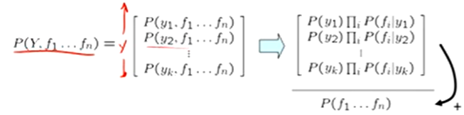
    • P(Y, F₁ … F_n) = P(Y) ∏ P(F_i | Y)

  • we only have to specify how each feature depends on the class

Inference for Naive Bayes

• compute posterior distribution over label variable Y

  • Step 1: get joint probability of label and evidence for each label

  • Step 2: sum to get probability of evidence

  • Step 3: normalize by dividing step 1 by step 2

Estimates of local conditional probability tables:

• P(Y), the prior over labels

• P(F_i | Y) for each feature (evidence variable)

• These probabilities are collectively called the parameters of the model and are denoted by θ

  

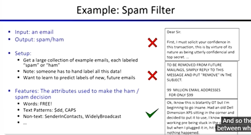
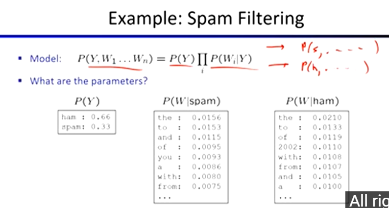
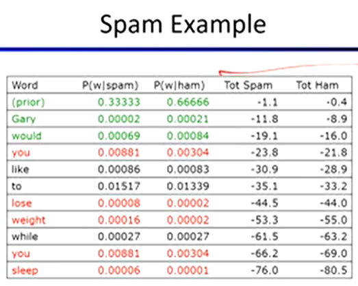
Naive Bayes for Text:

• bag-of-words Naive Bayes

  • features: W_i is the word at position i

  • as before: predict label conditioned on feature variables

  • as before: assume features are conditionally independent given label

  • new: each W is identically distributed

• generative model:

  • P(Y, W₁ … W_n) = P(Y) ∏ P(W_i | Y)

• “tied” distributions

  • usually, each variable gets its own conditional probablity distribution P(F | Y)

    • in bag-of-words model:

      • each position is identically distributed

      • all positions share the same conditional probs P(W | Y)

Training and Testing

• Empirical Risk Minimization

  • basic principle of ML

  • we want the model that does best on the true test distribution

  • don’t know the true distribution so pick the best model on our actual training set

  • finding “the best” model on the training set is phrased as an optimization problem

Data: labeled instances

• ex. emails marked spam

• training set

• held out set

• test set

Features: attribute-value pairs which characterize each x

Experimentation cycle:

• learn parameters on training set

• tune hyperparameters on held-out set

• compute accuracy of test set

• never “peek” at the test set

Evaluation: as many metrics as possible

• accuracy: fraction of instances predicted correctly

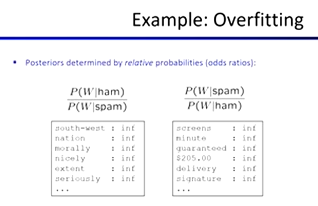
Overfitting and generalization

• want a classifier which does well on test data

• overfitting:

  • fitting the training data very closely, but not generalizing well

Parameter Estimation

• estimating the distribution of a random variable

• elicitation: ask a human

• empirically: use training data

  • for each outcome x, look at the empirical rate of that value

    • P_ML(x) = count(x) / total samples

  • this is the estimate that maximizes the likelihood of the data

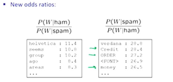
Laplace Smoothing

• Laplace’s estimate

  • pretend you saw every outcome once more than you actually did

    • P_LAP(x) = [c(x) + 1] / [Σ_x(c(x) + 1)] = [c(x) + 1] / [N + |X|]

  • pretend you saw every outcome an extra k times

    • P_LAPk(x) = [c(x) + k] / [N + k|X|]

Tuning on Held-Out Data

• parameters: the probabilities P(X | Y), P(Y)

• hyperparameters: the amount or type of smoothing to do, k, a

Features

• need more features to reduce errors

• can add these information sources as new variables in the NB model

Perceptrons & Logistic Regression

Linear Classifiers

• inputs are feature values

• each feature has a weight

• sum is the activation

  • activation_w(x) = Σ w_i ⋅ f_i(x) = w ⋅ f(x)

• if the activation is

  • positive, output +1

  • negative, output -1

Weights

• binary case: compare features to a weight factor

• learning: figure out the weight vector from examples

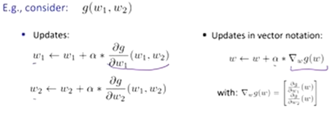
• Updates:

Binary Decision Rule

• in the space of feature vectors

  • examples are points

  • any weight factor is a hyperplane

  • one side corresponds to Y = +1

  • other corresponds to Y = -1

Binary Perceptron:

• start with weights = 0

• for each training instance:

  • classify with current weights

    • if correct, no change

      • correct if y = y*

    • if wrong, adjust the weight vector

      • add or subtract the feature vector

        • subtract if y* is -1

• w’ = w + y* ⋅ f

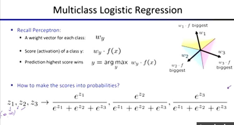
Multiclass Decision Rule

• if we have multiple classes (ex. 3)

  • a weight factor for each class: w_y

  • score (activation) of a class y: w_y ⋅ f(x)

  • prediction highest score wins: y = arg max w_y ⋅ f(x)

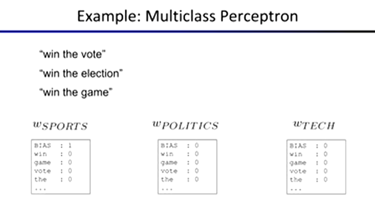
Multiclass Perceptron:

• start with all weights = 0

• pick up training examples one by one

• predict with current weights

  • y = arg max_y w_y ⋅ f(x)

• if correct, no change

  • correct if y = y*

• if wrong, lower score of wrong answer, raise score of right answer

  • w_y = w_y - f(x)

  • w_y* = w_y* + f(x)

Properties of Perceptrons

• separability

  • true if some parameters get the training set perfectly correct

• convergence

  • if the training is separable, the perceptron will eventually converge (binary case)

• mistake bound

  • the maximum number of mistakes (binary case) related to the margin or degree of separability

    • mistakes < k / s²

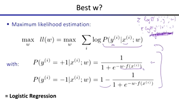
Deterministic Decision

• perceptron scoring: z = w ⋅ f(x)

  • if z = w ⋅ f(x) is very positive → want probability going to 1

  • if z = w ⋅ f(x) is very negative→ want probability going to 0

• sigmoid function

  • Ø(z) = 1 / (1 + e^-z)

Multiclass Logistic Regression

Optimization & Neural Networks

Hill Climbing

• start wherever

• repeat: move to the best neighbouring state

• if no neighbours better than current, quit

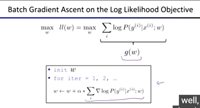
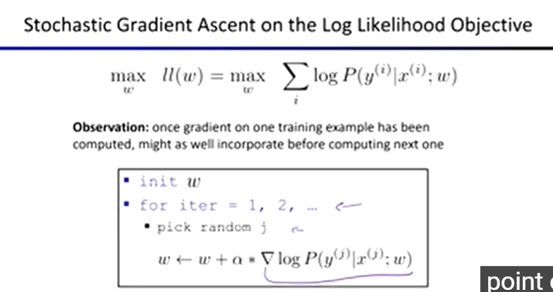
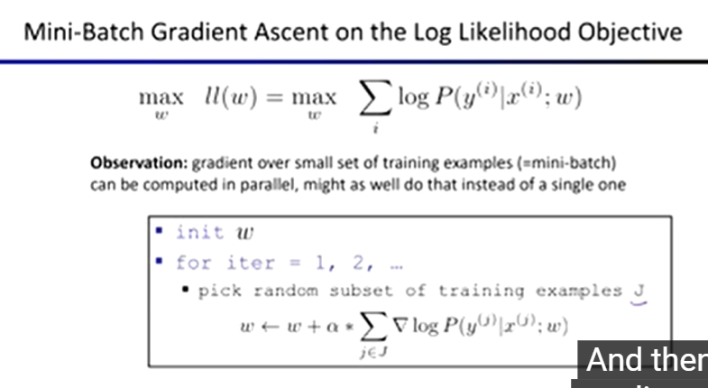
Optimization:

• ie: how do we solve

  • max_w ll(w) = max_w ∑ logP(y⁽ⁱ⁾ | x⁽ⁱ⁾ ; w)

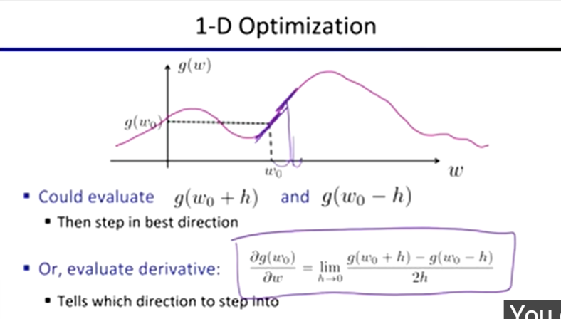
In higher-dimension cases …

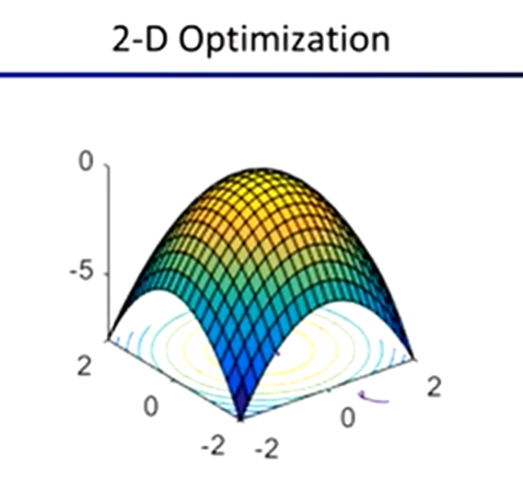
Gradient Ascent

• perform update in uphill direction for each coordinate

• the steeper the slope (the higher the derivative), the bigger the step for that coordinate

• start somewhere

  • repeat: take a step in the gradient direction

• Steepest direction: ∆ = ∇g / |∇g|

• procedure:

  • init w

  • for iter = 1, 2, …

    • w ← w + a * ∇g(w)

      • where a is the learning rate

Neural Networks:

• properties

  • universal function approximators

    • a two-layer neural network with a sufficient number of neurons can approximate any continuous function to any desired accuracy

  • practical considerations

    • can be seen as learning the features

    • large number of neurons

      • danger for overfitting

Multi-class Logistic Regression: a special case of neural network

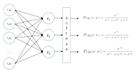
• each one does a calculation that looks like this:

  

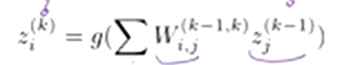
• g = nonlinear activation function

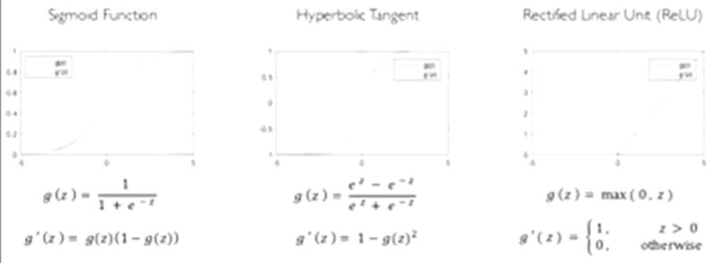
Common Activation Functions

Computing Derivatives:

• if neural network f is not in any of the tables…

  • chain rule!

    • if f(x) = g(h(x))

    • then f’(x) = g’(h(x))h’(x)

Automatic differentiation software:

• only need to program the function g(x, y, w)

• can automatically compute all derivatives

Decision Trees

Inductive Learning

• learn a function from examples

  • input-output pairs (x, g(x))

  • ex. x is an email and g(x) is spam / ham

• problem

  • given hypothesis space H

  • given a training set of examples X

  • find a hypothesis h(x) such that h ~ g

• includes:

  • classification (outputs = class labels)

  • regression (outputs = real numbers)

• Curve fitting (regression, function approximation)

  

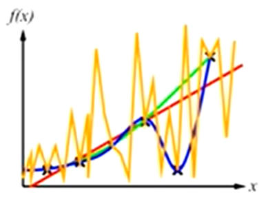
  • most algorithms favour consistency over simplicity

  • parabola has a bigger hypothesis space than a line

    • therefore overfitting is more likely in a parabola

  • Occam’s Razor:

    • try to find the simplest explanation of your data

  • ways to operationalize “simplicity”

    • reduce the hypothesis space

      • assume more

      • have fewer/better features

    • regularization

      • smoothing

Decision Trees

• compact representation of a function

  • truth table

  • conditional prob table

  • regression values

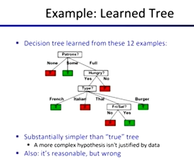
• true function

  • realizable in ff

Hypothesis Spaces

• how many distinct decision trees with n boolean attributes?

  • 2^{2^n}

• how many tress of depth 1 (decision stumps)?

  • 2²n = 4n

• a more expressive hypothesis space increases…

  • chance that target function can be expressed (good)

  • number of hypotheses consistent with training set (bad)

  • quality of predictions

Decision Tree Learning

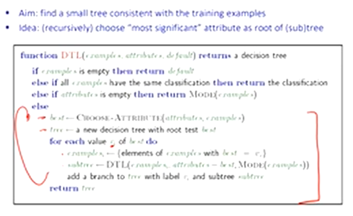
Choosing an Attribute

• a good attribute splits the examples into subsets that are (ideally) “all positive” or “all negative”

Information

• information answers questions

  • the more uncertain about the answer initially, the more information in the answer

  • scale: bits

    • Ans to boolean question with prior <1/2, 1/2>

      • 0 or 1 is only 1 bit being sent

    • Ans to 4-way question with prior <1/4, 1/4, 1/4, 1/4>

      • 2 bits

    • Ans to 4-way question with prior <0, 0, 0, 1>

      • 0 bits

    • Ans to 3-way question with prior <1/2, 1/4, 1/4>

      • ½ + ½ + ½ on average

• a probability p is typical of

  • a uniform distribution of size 1/p

  • a code of length log 1/p

Entropy

• general ans: if prior is <p₁, …, p_n>

  • H((p₁, …, p_n)) = E_plog₂1/p_i

    • = Σ -p_ilog₂p_i

• also called the entropy of the distribution

  • more uniform = higher entropy

  • more values = higher entropy

  • more peaked = lower entropy

  • rare values almost “don’t count”

• for each split, compare entropy before and after

  • difference is the information gain

• expected entropy:

  • weighted by the number of examples

    

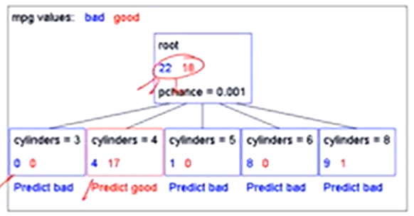
Find the first split:

• look for information gain for each attribute

• note that each attribute is correlated with the target

Decision Stump

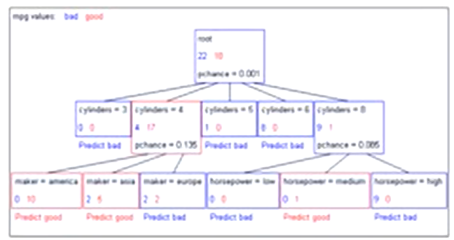
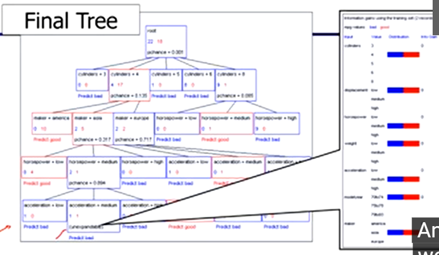
Significance of a Split

• starting with:

  • three cars with 4 cylinders, from Asia, with medium HP

  • 2 bad MPG

  • 1 good MPG

• shouldn’t split if the counts are so small that they could be due to chance

• a chi-squared test can tell us how likely it is that deviations from a perfect split are due to chance

• each split will have a significance value, P_CHANCE

Pruning:

• build the full decision tree

• begin at the bottom of the tree

• delete splits in which P_CHANCE > MaxP_CHANCE

• continue working upward until there are no more prunable nodes