Chapter 9: Inferences from Two Samples
Section 9.2 Two Means: Independent Samples
Two Independent / Dependent Samples
Independent Samples: when the sample values from one population are not related to or somehow naturally paired or matched with the sample values from the other population
Dependent Samples (matched pairs): when the samples are somehow matched, where the matching is based on some inherent relationship
Each pair of sample values consists of two measurements from the same subject, such as…
before/after data
…or each pair of sample values consists of matched pairs (such as husband/wife data) where the matching is based on some meaningful relationship
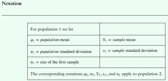
Assumptions
The two samples are independent
Both samples are simple random samples
Either or both of these conditions is satisfied: The two sample sizes are both large (n1 > 30) and from (n2 > 30) or both samples come from populations having normal distributions
Comments:
Do not pool variances
df = smaller of n1 - 1 and n2 - 1
Hypothesis Test Statistic for Two Mean: Independent Samples
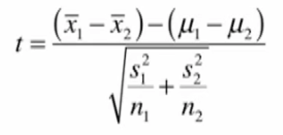
= claimed population mean
Very often, the two claimed population means will be equal to each other
Confidence Variable
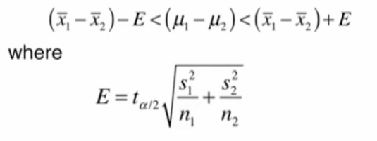
and the degrees of freedom is determined as the smaller of (n1 - 1) and (n2 - 1)
Example 1
Many studies have been conducted to test the effects of marijuana use on mental abilities. In one such study, groups of light and heavy users of marijuana in college were tested for memory recall, with the results given in the following table.
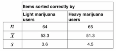
The light users had a mean of 53.3
The heavy users had a mean of 51.3
Is this difference significant?
Take into account:
The sample sizes
The magnitude of the difference
etc.
Since we can’t do all of this in our minds, we use a formal structure of a hypothesis test
Use a 0.01 significance level to test the claim that the population of heavy marijuana users has a lower mean than the light users. Should marijuana use be of concern to college students?
Is 1 greater than 2?
We know that 53.3 is a number greater than 51.3 BUT does this suggest that the light marijuana users greater than the heavy marijuana users?
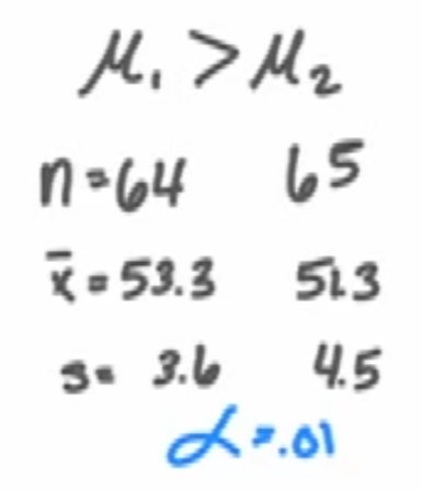
The picture above contains the key components needed to procede
Steps for Testing Hypotheses:
Identify the claim and put it into symbolic form (\mu_1>\mu_2)
Put the opposite of the claim in symbolic form ()
Look at the previous steps and identify the alternative hypothesis
H1: \mu_1>\mu_2 (alternative hypothesis)
H0: (null hypothesis)
t = 2.790
P-value
for t = 2.79 and df = 63:
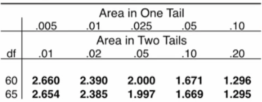
The table is a right-tailed test
“df” is found through finding the degrees of freedom of both samples and choosing the smallest number
2.79 is father off to the left (bigger than any of the bolded values) on the table
Based on this, we can include the P-value is less than 0.005
When using the traditional approach…
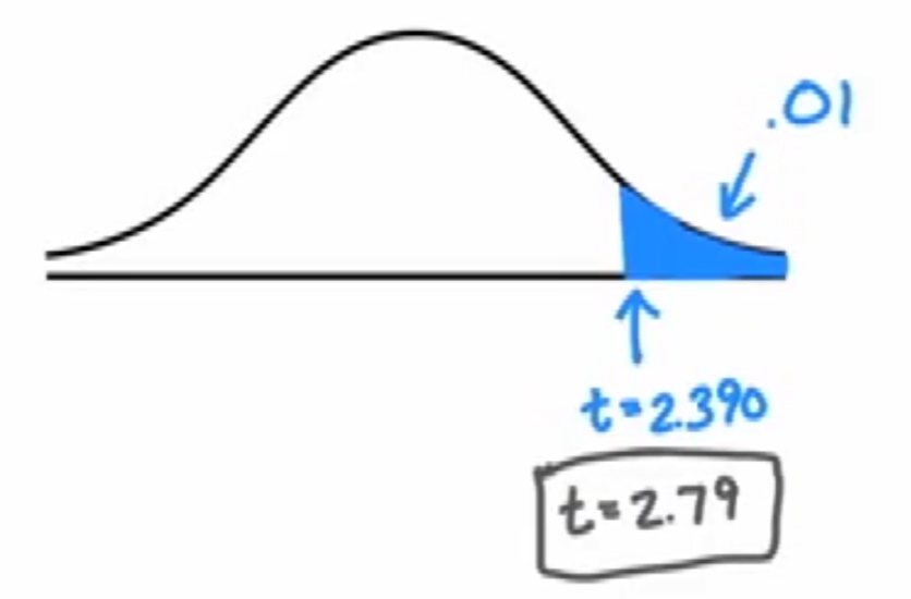
The critical value could be looked up from the table above the bell-curve
Look at .01 under “Area in One Tail” since the significance level is .01
Picking either 2.390 OR 2.385 will leave the same conclusion, which is…
To therefore REJECT the null hypothesis (H0) because the t-score falls in the critical region
There is sufficient evidence to support the original claim that heavy marijuana users scored lower than light marijuana users
98% Confidence Interval (if we were to proceed with this)
and the degrees of freedom is determined as the smaller of (n1 - 1) and (n2 - 1)
This provides the confidence interval
Since this interval excludes zero, we REJECT the null hypothesis
Section 9.3 Two Dependent Samples (Matched Pairs)
Two Independent / Dependent Samples
Independent Samples: when the sample values from one population are not related to or somehow naturally paired or matched with the sample values from the other population
Dependent Samples (matched pairs): when the samples are somehow matched, where the matching is based on some inherent relationship
Each pair of sample values consists of two measurements from the same subject, such as…
before/after data
…or each pair of sample values consists of matched pairs (such as husband/wife data) where the matching is based on some meaningful relationship
Assumptions
The two samples are dependent (Matched pairs)
Both samples are simple random samples
Either or both of these conditions is satisfied: The two sample sizes are both large (n1 > 30) and from (n2 > 30) or both samples come from populations having normal distributions
Hypothesis Test Statistic for Matched Pairs of Sample Data
where degrees of freedom = n - 1
d = individual difference between the two values in a single matched pair
= The mean of the differences from the population of matched data // mean value of the differences d for the population of all matched pairs of data
= mean value of the differences d for the paired sample data
sd = standard deviation of the differences d for the paired sample data
n = number of pairs of sample data
Confidence Intervals for Matched Pairs
\overline{d}-E<\mu_{d}<\overline{d}+E
where
Here ta/2 is the critical value obtained using Table A-3 with n - 1 degrees of freedom
Example 1
The following table consists of five actual low temperatures and the corresponding low temperatures that were predicted five days earlier
1 | -5 | -5 | 23 | ||
Forecast low | 16 | 16 | 20 | 22 | 15 |
-15 | -21 | -25 | 1 |
Use a 0.05 significance level to test the claim that there is a difference between the actual low temperatures and the low temperatures that were forecast five days earlier.
We’re saying that because we’re operating under the assumption that the mean difference is equal to 0
Since the claim was that there is a difference between the actual low and the forecast low…
That’s really the claim that
If we’re saying that that is NO difference between the actual low and the forecast low, the claim would be
Therefore…
H1 (alternative hypothesis) :
H2 (null hypothesis) :
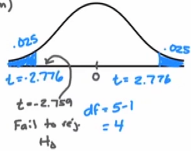
H1 : (claim)
H0 :
t = -2.759
Because t is not in the critical region, we fail to reject the null hypothesis
“I don’t have sufficient evidence to support the claim that the mean difference is different than 0”
For the Confidence Interval…
We use
n = 5
\overline{d}-E<\mu_{d}<\overline{d}+E
-13.2-13.3<\mu_{d}<-13.2+13.3
-26.5<\mu_{d}<0.1
We end up with this 95% confidence interval
95% confident that the limits of -26.5 and 0.1 contain the true population mean difference
The confidence interval limits do contain 0, suggesting that it might well be that the population mean difference is the value of 0
Indicating that there is not a significant difference between actual temperature and forecast temperatures
If the
What design principle is stressed for experiments or observational studies?
A. When using paired data, keep the sample very small in order to keep the data manageable.
B. The methods for dependent samples can be used for any matched pairs.
C. Using two independent samples is the best choice for accurate results.
D. Using dependent samples with paired data is generally better than using two independent samples.