Comprehensive Guide to Integration and Accumulation

Defining the Integral: From Rate to Accumulation

Accumulation of Change

In the first half of Calculus (Differential Calculus), we focused on the Derivative, which tells us the instantaneous rate of change of a function. Now, we reverse the process. If we know the rate of change, how do we find the total change or accumulation?

Concept Integration: The Integral (denoted by $\int$) is essentially the "Antiderivative."

• Derivative: Rate of change per unit (slope).
• Integral: Accumulation of change over an interval (area).

Geometrically, the Definite Integral represents the net signed area bounded by the graph of a function $f(x)$ and the $x$-axis between two $x$-values.

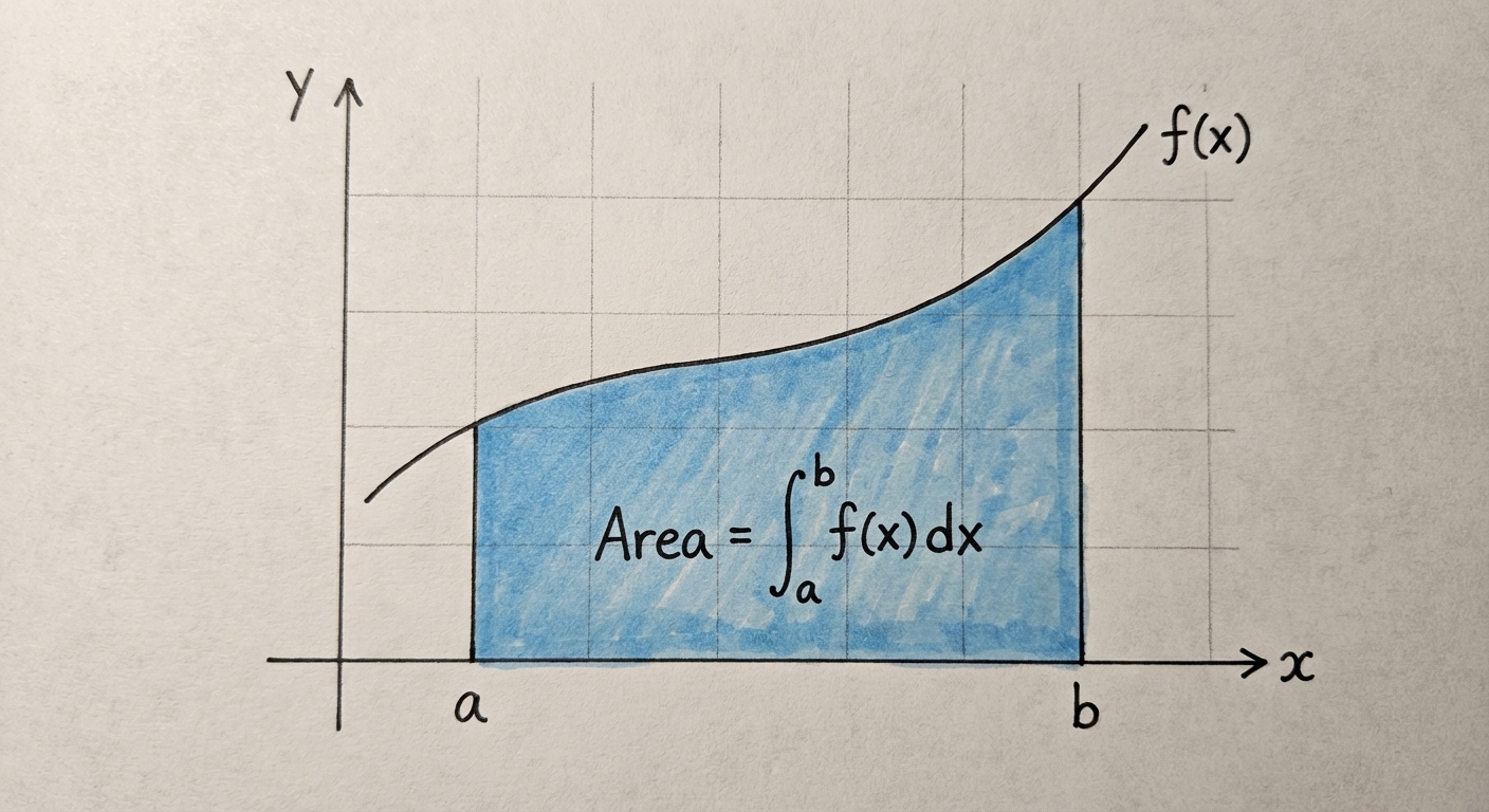
The Notion of Net Signed Area

When calculating integrals, "area" has a sign:

• Positive Area: Region above the $x$-axis.
• Negative Area: Region below the $x$-axis.
• Net Accumulation: The sum of positive areas minus the absolute value of negative areas.

Riemann Sums: Approximating Area

Before we have exact formulas, we estimate the area under a curve using shapes we know: rectangles (and trapezoids). This estimation method is called a Riemann Sum.

The General Concept

To estimate the area under a curve $f(x)$ from $a$ to $b$:

1. Slice the region into $n$ subintervals (strips).
2. Draw a rectangle in each strip.
3. Calculate Area $= \text{width} \times \text{height}$.
4. Sum the areas.

As the number of rectangles ($n$) approaches infinity ($
\to \infty$), the width of each rectangle ($
\Delta x$) approaches zero, and the approximation becomes the exact integral:

$\int<em>a^b f(x) dx = \lim</em>{n \to \infty} \sum<em>{i=1}^{n} f(x</em>i) \Delta x$

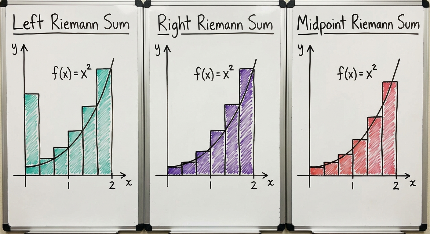
Types of Riemann Sums

When building these rectangles, the width is usually determined by the interval on the $x$-axis, but the height differs based on which point of the function we use.

1. Left Riemann Sum (LRAM)

• Height: The value of $f(x)$ at the left endpoint of the subinterval.
• Construction: The top-left corner of the rectangle touches the curve.
• Behavior: Underestimates increasing functions; Overestimates decreasing functions.

2. Right Riemann Sum (RRAM)

• Height: The value of $f(x)$ at the right endpoint of the subinterval.
• Construction: The top-right corner of the rectangle touches the curve.
• Behavior: Overestimates increasing functions; Underestimates decreasing functions.

3. Midpoint Riemann Sum (MRAM)

• Height: The value of $f(x)$ at the exact middle $x$-value of the subinterval.
• Accuracy: Usually more accurate than LRAM or RRAM for the same number of rectangles.

Trapezoidal Sums

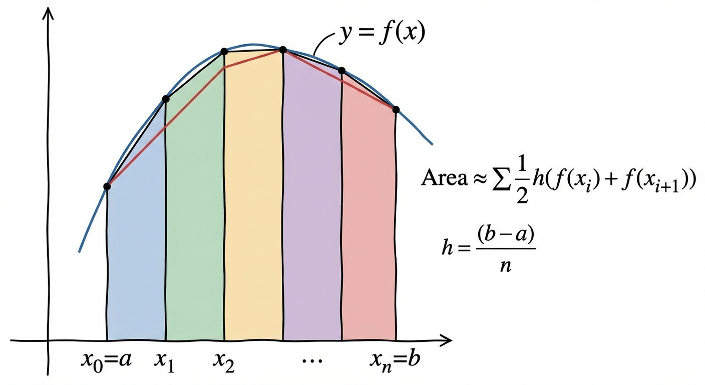
Instead of flat-topped rectangles, we can use trapezoids to connect the function values. This often provides a much better approximation because the geometric shape "hugs" the curve.

Area of a Trapezoid Formula:
$A = \frac{1}{2}(b<em>1 + b</em>2)h$

• In calculus context: $b<em>1$ and $b</em>2$ are the function heights ($y$-values), and $h$ is the interval width ($
  \Delta x$).
• Formula: $\frac{1}{2}(f(x<em>1) + f(x</em>2)) \cdot \Delta x$

Working with Tabular Data

On the AP Exam, you are frequently given a table of values rather than a function equation. You must pay attention to whether the intervals (widths) are equal or unequal.

Example: Tabular Riemann Sum

Task: Estimate $\int_0^7 H(t) dt$ using different methods.

1. Left Sum (LRAM)
Use the left $y$-value for height. Widths are differences in $t$ ($2-0=2$, $4-2=2$, $7-4=3$).

• Rect 1: Width $2$, Height $1$ $\rightarrow 2(1)$
• Rect 2: Width $2$, Height $6$ $\rightarrow 2(6)$
• Rect 3: Width $3$, Height $10$ $\rightarrow 3(10)$
• Total: $2 + 12 + 30 = 44$

2. Right Sum (RRAM)
Use the right $y$-value for height.

• Rect 1: Width $2$, Height $6$ $\rightarrow 2(6)$
• Rect 2: Width $2$, Height $10$ $\rightarrow 2(10)$
• Rect 3: Width $3$, Height $15$ $\rightarrow 3(15)$
• Total: $12 + 20 + 45 = 77$

3. Trapezoidal Sum
Use the average of the two heights.

• Trap 1: $\frac{1}{2}(1+6)(2) = 7$
• Trap 2: $\frac{1}{2}(6+10)(2) = 16$
• Trap 3: $\frac{1}{2}(10+15)(3) = 37.5$
• Total: $7 + 16 + 37.5 = 60.5$

4. Midpoint Sum (MRAM) - Note on Data

• To perform a midpoint sum, we need the data point exactly in the middle. Looking at the interval $t=0$ to $t=4$, the midpoint is $t=2$.
• One large rectangle from 0 to 4: Width is $4$. Midpoint height is at $t=2$, which is $H(2)=6$.
• Area: $4(6) = 24$. (We cannot calculate the rest of the table because we don't have a midpoint value between 4 and 7).

Antiderivatives & Indefinite Integrals

When we find an integral without limits (bounds), it is called an Indefinite Integral. This represents the family of functions whose derivative is the given function.

The Power Rule for Integration

Recall the Power Rule for derivatives: Multiply down, subtract one. For integration, we do the inverse!

Rule: Add one to the exponent, then divide by the new exponent.

$\int x^n dx = \frac{x^{n+1}}{n+1} + C$
(where $n \neq -1$)

The "+ C" is Non-Negotiable!
Since the derivative of a constant is zero (e.g., $\frac{d}{dx}[x^2 + 5] = 2x$ and $\frac{d}{dx}[x^2 - 100] = 2x$), we don't know what constant existed originally. We simply add $+C$, the Constant of Integration.

Examples:

1. Simple: $\int 2x dx = \frac{2x^2}{2} + C = x^2 + C$
2. Fractional Powers: $\int \sqrt{x} dx = \int x^{1/2} dx = \frac{x^{3/2}}{3/2} + C = \frac{2}{3}x^{3/2} + C$
3. Basic Trig: You must reverse your derivative memory.
   • $\int \cos(x) dx = \sin(x) + C$
   • $\int \sin(x) dx = -\cos(x) + C$ (Watch the sign!)
   • $\int \sec^2(x) dx = \tan(x) + C$

The Fundamental Theorem of Calculus (FTC)

This is the bridge connecting Differential Calculus (rates) and Integral Calculus (accumulation).

FTC Part 1: The Evaluation Theorem

If $f$ is continuous on $[a, b]$ and $F$ is an antiderivative of $f$, then:

$\int_a^b f(x) dx = F(b) - F(a)$

Evaluating Definite Integrals:

1. Find the antiderivative equation.
2. Plug in the upper bound ($b$).
3. Plug in the lower bound ($a$).
4. Subtract: (Upper) - (Lower).

Example: Evaluated $\int_2^3 2x dx$

• Antiderivative: $x^2$
• Plug in 3: $3^2 = 9$
• Plug in 2: $2^2 = 4$
• Result: $9 - 4 = 5$
• (Note: The $+C$ cancels out in definite integrals, so we ignore it.)

FTC Part 2: Derivatives of Integrals

This part states that differentiation and integration are inverse processes. If you take the derivative of an accumulation function:

$\frac{d}{dx} \int_a^x f(t) dt = f(x)$

Chain Rule Variance (Crucial for AP):
If the upper limit is a function $g(x)$ rather than just $x$, you must apply the chain rule:

$\frac{d}{dx} \int_a^{g(x)} f(t) dt = f(g(x)) \cdot g'(x)$

Example:
$\frac{d}{dx} \int_5^{x^3} \sin(t) dt = \sin(x^3) \cdot (3x^2)$

Properties of Definite Integrals

Manipulating integrals algebraically is a key skill.

1. Zero Width: $\int_a^a f(x) dx = 0$
2. Reversal: $\int<em>a^b f(x) dx = - \int</em>b^a f(x) dx$ (Switching bounds flips the sign)
3. Additivity: $\int<em>a^c f(x) dx = \int</em>a^b f(x) dx + \int_b^c f(x) dx$
4. Linearity: $\int<em>a^b [k \cdot f(x) + g(x)] dx = k\int</em>a^b f(x)dx + \int_a^b g(x)dx$

Advanced Integration: Method of Substitution (U-Sub)

What if the integral looks basically impossible, or is a composite function? This is the reverse of the Chain Rule.

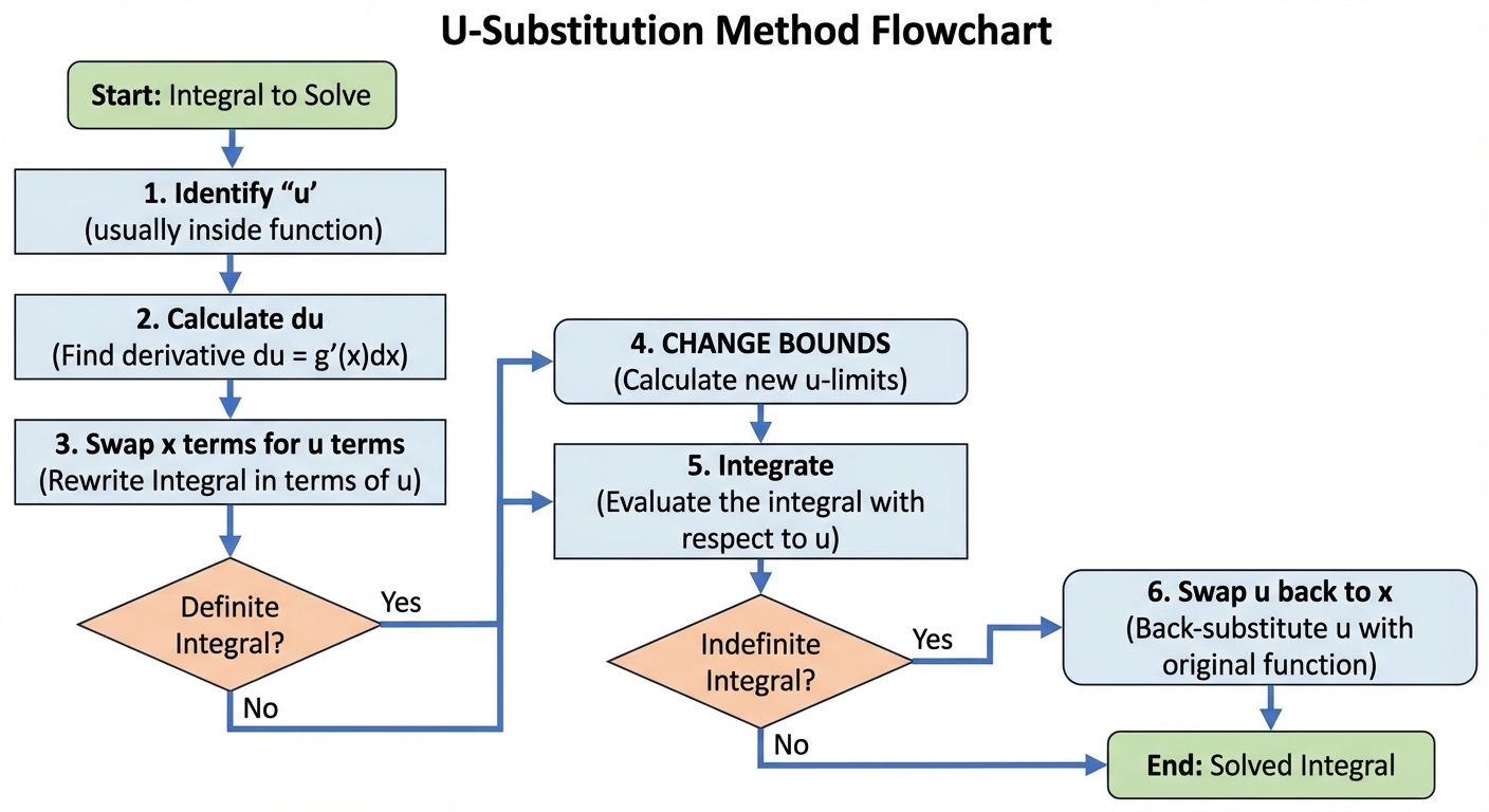
The Strategy:

1. Choose $u$: Look for an "inside" function whose derivative is also present (or close to present) in the integrand.
2. Differentiate: Find $du = f'(x) dx$.
3. Solve for $dx$: Isolate $dx$ to substitute it back into the integral.
4. Substitute: Rewrite the entire integral in terms of $u$. All $x$'s must go!
5. Integrate: Use basic power rules on $u$.
6. Back-Substitute (Indefinite only): Replace $u$ with the original $x$ expression.

Definite Integrals & U-Sub (Change Calculation)

Important: When doing a definite integral with U-Sub, you should change the bounds from $x$-values to $u$-values using your $u$ equation. Then you never have to go back to $x$!

Worked Example: $\int_0^1 2x(x^2 + 1)^3 dx$

1. Identify $u$: $u = x^2 + 1$ (This is the inside function).
2. Differentiate: $du = 2x dx$.
3. Match: We have a $2x dx$ in the problem! So we can swap $2x dx$ for $du$.
4. Change Bounds:
   • If $x = 0$, $u = 0^2 + 1 = 1$.
   • If $x = 1$, $u = 1^2 + 1 = 2$.
   • New integral: $\int_1^2 u^3 du$.
5. Integrate: $\left[ \frac{u^4}{4} \right]_1^2$
6. Evaluate: $\frac{2^4}{4} - \frac{1^4}{4} = \frac{16}{4} - \frac{1}{4} = \frac{15}{4}$.

Common Mistakes & Exam Pitfalls

• Forgetting $+C$: In indefinite integrals, omitting the constant of integration is an instant point deduction.
• Uneven Tables: Students often assume $\Delta x$ is constant in tables. Always calculate the specific width for each interval (e.g., $2, 2, 3$ in the earlier example).
• Trapezoid Formula: A common error is summing the heights and dividing by 2 at the end. You must calculate the area of each trapezoid individually if widths vary.
• FTC Chain Rule: When taking the derivative of an integral $\frac{d}{dx}\int_a^{x^2}…$, students forget to multiply by the derivative of the upper limit ($2x$).
• Total Change vs. Net Change: $\int<em>a^b v(t) dt$ gives displacement (net change in position). $\int</em>a^b |v(t)| dt$ gives total distance traveled. Know the difference!