ECON Midterm Prep
Introduction to Markets and Demand
Understanding the basics of demand in markets.
Overview of the upcoming classes: supply and a combination of supply and demand.
Discussion about the essential nature of markets: reliance on governments vs. markets solving problems independently.
Introduction of economic models as simplified versions of reality.
Important relationships include price and quantity demanded.
Fundamental Model of Demand
Introduction to basic demand model and assumptions, particularly perfect competition.
Discussion of real-world applicability versus theoretical ideals.
Noted variances from the perfect competition model and implications.
Class Structure and Tools Utilized
Use of an iClicker for class participation and questions.
Adjustment in assignment due dates and handling of technical issues with platforms like Brightspace.
Opportunity Cost and Time Allocation Exercise
Example scenario: allocating time between walking the dog and playing video games.
Understanding the concept of opportunity cost in a time management context.
Example Calculations:
1 hour = 1 dog walk
2 hours = 1 video game session
Total capacity limited to 10 hours.
Different scenarios (A, B, C, D, E) questioning efficiency and feasibility of time allocation.
Slopes of curves depicting opportunity costs.
Marginal Cost and Decision-Making Scenario
Vincent's handcrafted tables: pricing, production costs, and optimal output analysis.
Calculation of marginal costs for each table produced:
First table: $1000
Second table: $1500
Adds $500 for each additional table.
To maximize profit: where marginal cost meets marginal revenue ($3000).
Conclusion: production of five tables maximizes profit without exceeding marginal cost.
Demand vs. Quantity Demanded
Clarification of quantity demanded as movement along the demand curve.
Differentiation of demand as a shift in the entire curve based on external factors.
Key points to observe:
The demand curve is downward sloping, indicating an inverse relationship between price and quantity demanded.
Shifts to the left or right based on external factors affecting demand, such as income changes, tastes, or price of substitutes and complements.
Market Definition & Competitive Assumptions
Market is defined as the sum of buyers and sellers of a good/service.
Perfect competition assumes many buyers/sellers, leading to price-taking behavior.
The invisible hand concept—market forces leading to efficient allocation of resources.
Limitations of the Market Model
Potential market failures requiring government intervention:
Externalities (e.g., social costs of smoking).
Labor markets and minimum wage discussions.
Importance of societal choice and intervention for equitable distribution of resources (e.g., housing, food).
Factors Determining Demand
Various factors influencing individual demand for coffee (or other goods):
Consumer income.
Tastes and preferences.
Price of complementary and substitute goods.
Understanding the relationship between the good's price and quantity demanded, leading to the law of demand:
As price increases, quantity demanded decreases, and vice versa.
Demand Curve Representation
Illustration through graphs, equations, and tables to express demand:
Example demand equation: $Q_d = 54 - 7P$.
Calculation of quantity demanded at different price points with results indicating the downward slope of the curve.
Total and marginal benefit illustrated through utility and consumer choices.
Diminishing Marginal Benefit
Concept illustrated through human experience with goods (e.g., Timbits).
Total utility increases while marginal utility diminishes with each additional unit consumed.
Application of diminishing marginal benefit to demand curve construction.
Market Demand Construction
Combining individual demand for coffee at various price points to generate a market demand curve.
Understanding how demand responds to pricing dynamics and external factors.
Expectations and Behavioral Economics
Influence of consumer expectations about future prices on present demand.
Example scenarios illustrating how anticipation of price changes influences current purchasing behavior.
Network Effects and Congestion Effects
Explanation of how social factors and prevalence of usage by others impact individual demand.
Examples of how too much demand leads to congested experiences affecting decisions (e.g., driving).
Impact of Changes in Population
Correlation between population growth and market demand for goods like housing.
Real-world context regarding the housing market in Halifax amidst population changes due to the pandemic.
Conclusion and Summary of Key Points
Differentiation between shifts (changes in demand) and movements along the demand curve (changes in quantity demanded).
Importance of various external factors that can shift the demand curve, including substitutes, complements, and future expectations.
Purchasing Goods and Services
Nature of Consumption: Students are encouraged to engage in purchasing commonly needed goods and services, such as:
Books
Clothing
Legal Services
Traveling
Law of Demand:
Definition: The principle that states the higher the price of a good, the less likely consumers are to buy it.
Reasons for the Law:
Goods may be too expensive.
Consumers may not value the goods highly enough to purchase them.
Production and Supply Side
Transitioning to the Production Side:
Observation: Everyone, through previous summer jobs or experiences, has likely engaged in production activities, e.g., working in a restaurant or on a farm.
Understanding Supply:
Definition: Supply refers to the availability of goods and services being produced and offered to the market.
Examples of Supply:
Producing coffee and selling it.
Growing wheat and selling it.
Includes the supply of labor, where workers provide their labor services in return for wages.
Labor Supply:
Concept: The higher the wages offered, the more workers will be willing to supply their labor.
Individual Supply Curve:
Shape: The individual supply curve is typically upward sloping (positively sloped).
Explanation for Upward Slope:
As prices increase, producers are incentivized to supply more.
Market Supply Curves
Market Supply:
Combining individual supply curves to form a market supply curve by adding quantities at different price levels.
Movement vs. Shift in Curves:
Movement Along the Curve: Occurs when the price of a good changes, leading to a change in quantity supplied.
Shift of the Curve: Happens when external factors affect supply other than the price of the good itself, leading to an entire curve moving left or right.
Perfectly Competitive Market
Definition of Perfectly Competitive Market:
Characterized by:
Numerous consumers and producers.
Uniform (identical) goods.
Price-taking behavior – no single producer can influence the market price.
Free entry and exit of firms in the market.
Perfect information regarding prices.
Examples in Reality: While the model is insightful, not all markets exhibit these characteristics.
Wages and Labor Supply Hypothetical Example
Classroom Experiment on Labor Supply:
Experiment involved varying wages to gauge willingness to work for given hours.
Hypothetical Wage Increases:
At $5, students' interest varies.
At $20/hour and $250/hour, interest generally increases.
Law of Supply
Definition: The law of supply posits that as the price increases, the quantity supplied also increases, and vice versa.
Supply Curve Relation:
The supply curve confirms this relationship and is positively sloped.
Opportunity Cost and Labor Supply
Explanation of Opportunity Cost:
Higher wages lead generally to an increased willingness to work more hours.
However, there may be thresholds where additional work hours become less desirable due to other personal costs or recreational activities.
Experiments with Aggregating Labor Data
Example with individual workers’ responses:
Predictably, fewer workers generally lead to reduced efficiencies as more factors are additionally consumed or utilized inefficiently.
Cost Definitions
Fixed Cost:
Costs that remain constant regardless of the level of production, e.g., rent or salaries.
Variable Cost:
Costs that vary directly with the level of production, e.g., raw materials and hourly labor.
Profit Maximization
Concept: Businesses seek to maximize profits by producing where marginal revenue equals marginal cost.
Marginal Costs Explained:
Represents the extra cost incurred to produce one more unit.
Competitive Supply and Production Example
Marginal Cost's Connection to Supply Curve:
As costs rise, the quantity supplied increases.
The balance between marginal revenue and marginal costs dictates production levels in a competitive market setup.
Shift Factors for Supply Curve
Elements that shift the supply curve:
Changes in production costs or efficiency.
Variations in technology or input prices.
Substitutes vs. Complements in Production:
Production of one good can influence the production of another.
Expectations:
If prices are expected to rise, suppliers may reduce current output in anticipation of higher future prices.
Conclusion
Markets rely on both demand and supply concepts to determine equilibria and price levels, essential for understanding broader economic principles.
The relationships established in perfectly competitive markets provide a framework for understanding dynamics in less-than-perfect scenarios, which can be analyzed in future studies.
Economic Concepts of Supply and Demand
Increase in Supply
Key Concept: There is a clear relationship between price and quantity supplied.
At a given price, if marginal cost decreases (for instance), supply increases.
Example: If producing one unit incurs lower production costs (shift scenario), the quantity supplied of a good, like burgers, increases.
Depicted as a rightward shift in the supply curve.
Understanding Pricing and Demand
Change in Price Context: If the price point rises from $15 to $18, demand is expected to increase, potentially leading to higher production.
Supply Arising from Price Changes:
If only the price changes but costs remain the same, the supply will move along the curve, not shift.
Key Distinction: Shifts vs. Movements
Shifts in supply curves occur due to changes other than price (e.g., production costs).
Example: If costs decrease (e.g., worker wages lower), the supply curve shifts to the right.
Movements occur when price is the only factor that changes while maintaining production costs.
Market Economy vs. Planned Economy
Planned Economy (Ex-USSR example)
Definition: An economy where the government decides on production and distribution.
Critique:
Costly and Inefficient: Hard to determine what needs production, who should produce, and who should consume.
Lack of Incentives: Without profit motives, there are fewer incentives for innovation or cost reduction.
Outcomes: Poor allocation of resources may happen due to bureaucratic inefficiencies.
Market Economy
Adam Smith's Ideology: Free market mechanisms allow supply and demand to determine prices without major government intervention.
Belief in the 'invisible hand' of the market, suggesting that individual self-interests drive efficient outcomes.
Flexibility of Markets:
Workers may find jobs that correspond to their skill levels, but income may not always meet living costs.
Criticisms:
Markets can lead to income inequality and potentially ignore environmental consequences.
Example: Increased production may lead to pollution, as market forces alone do not ensure clean air or water.
Equilibrium in Market
Definition: The point where quantity demanded equals quantity supplied, resulting in stable prices.
Shifts in Demand and Supply:
When demand increases (demand curve shifts right), it typically results in higher prices and quantities supplied.
Conversely, an increase in supply (supply curve shifts right) leads to lower prices and higher quantities.
Market Adjustments:
If the market price is above equilibrium, excess supply (surplus) occurs; producers will lower prices to encourage sales.
If the price is below equilibrium, excess demand (shortage) occurs; consumers will bid prices up, resulting in higher equilibrium prices.
Mathematical Representation of Demand and Supply
Demand Equation
General Form:
Interpretation: For every $1 increase in price, quantity demanded decreases by 7.
Supply Equation
General Form:
Interpretation: For every $1 increase in price, quantity supplied increases by 10.
Finding Equilibrium Price and Quantity
Equilibrium Condition: implies
Rearranging gives:
Substituting back yields the equilibrium quantity.
Identifying and Resolving Surplus and Shortage
Surplus
Occurs when quantity supplied exceeds quantity demanded, prompting the market to lower prices.
Shortage
Occurs when quantity demanded exceeds quantity supplied, prompting the market to raise prices.
Market Condition Examples
Current market dynamics:
Shortage example: Lack of affordable housing while high market prices persist.
Surplus example: Excess amount of goods like clothes or food items leading to markdowns.
Revisiting Market Mechanics
Effect of Demand Shift: An increase in consumer preference for a good will shift the demand curve to the right, leading to more quantity sought at every price.
Effect of Supply Shift: A rise in raw material prices shifts the supply curve left, leading to a decrease in quantity supplied at existing prices.
Government Intervention Discussion
Rationale for Intervention: In cases of significant market failure (like monopolies, public goods, etc.), government actions are necessary to stabilize markets.
Examples of Government Intervention: Housing subsidies, regulations limiting price increases, and promoting competition to stabilize market conditions and ensure fair access.
Conclusion
Understanding these economic principles equips students with tools to analyze real-world markets and predict outcomes based on varying demand or supply conditions.
The balance between theoretical foundations, real-market implications, and the role of government is crucial in modern economic studies.
Overview of Elasticity in Economics
Definition of Elasticity
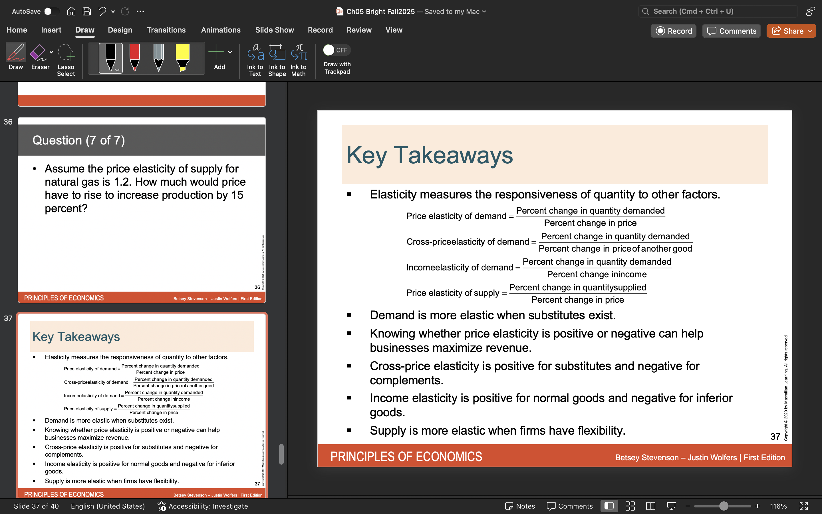
Refers to the responsiveness of quantity demanded or supplied to changes in other economic variables
Price Elasticity of Demand
Concept
Examines how consumption changes in response to price changes
Measures the sensitivity of demand relative to price changes
Shape of Demand Curve
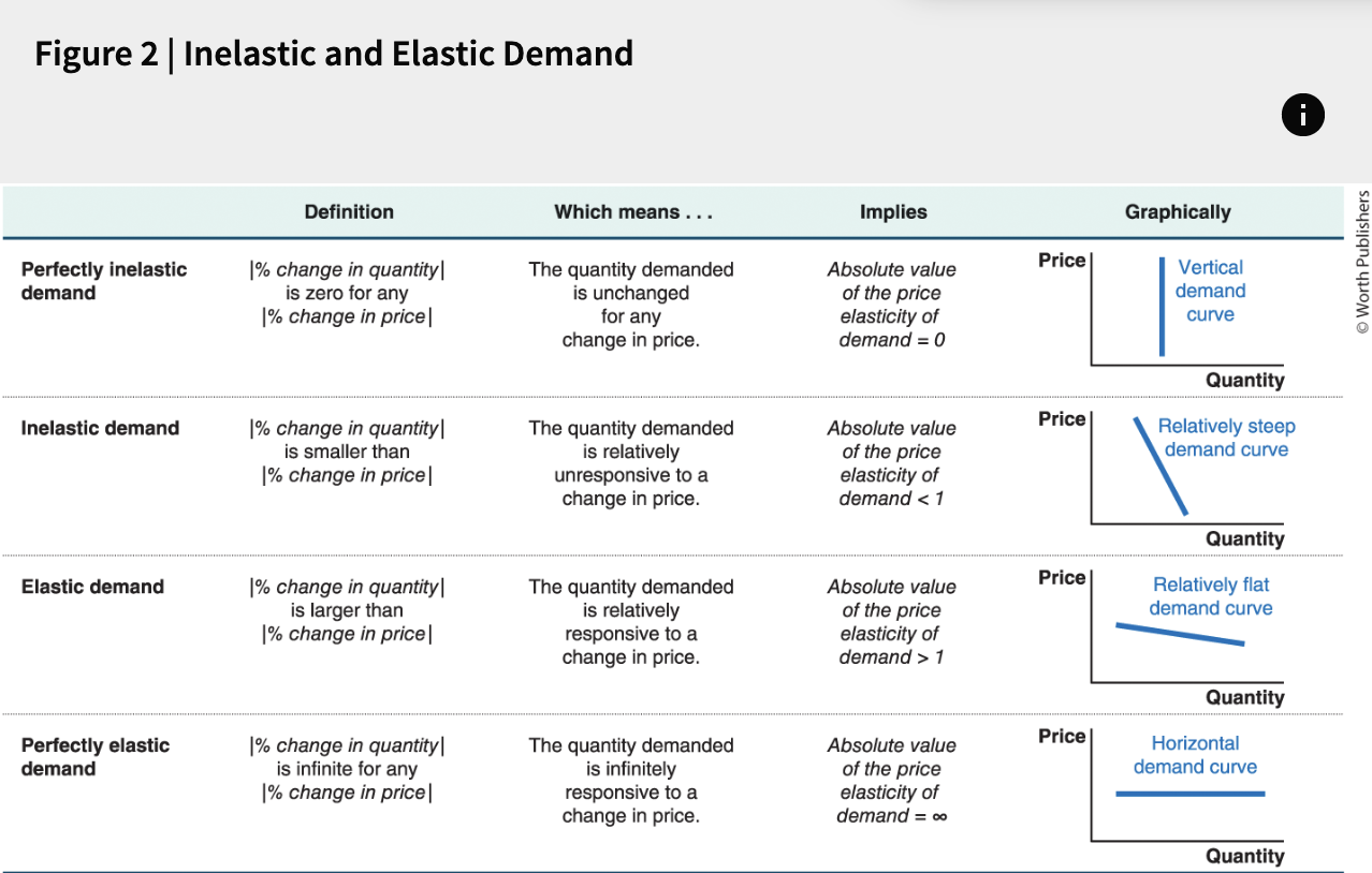
Flatter demand curves indicate more elastic demand
Steeper curves indicate less elastic (inelastic) demand
Calculating Price Elasticity of Demand
Formula:
Independent variable: price of the good
Dependent variable: quantity demanded
The price elasticity of demand is generally negative; however, we focus on the absolute value
Interpretation:
If the value is greater than 1, demand is elastic
If less than 1, demand is inelastic
Example: A 1% increase in price could lead to a 2% decrease in quantity demanded (elastic)
Extremes
Perfectly elastic demand (horizontal line, infinite responsiveness)
Perfectly inelastic (vertical line, zero responsiveness)
Revenue Implications of Price Elasticity
Inelastic Demand Example:
Example of pharmaceutical drugs: Consumers will purchase regardless of price
Implication:
Higher prices can lead to increased revenue if demand is inelastic
Example Calculation and Discussion
Calculation Example
Price elasticity of demand for air travel:
If elasticity is 4:
A 20% decrease in price leads to an 80% increase in quantity demanded (4 x 20% = 80%)
If price increases by 11%, quantity demanded increases by 40%
Check Understanding of Calculation Concepts
Ensure comprehension of calculations such as or
Cross Price Elasticity of Demand
Definition
Measures the responsiveness of demand for one good when the price of another good changes
Complementary Goods:
If the price of one good increases, the demand for the complement decreases
Example: Price of hot dogs rises, demand for buns falls
Results in negative cross price elasticity
Substitutes Example:
Price increase in one product leads to demand increase in another
Example: Price of tea increases, demand for coffee rises
Results in positive cross price elasticity
Significance of Sign:
Understanding if goods are substitutes or complements based on sign of elasticity
Income Elasticity of Demand
This elasticity measures how quantity demanded changes as income changes.
Normal Goods:
is positive
Inferior Goods:
Negative income elasticity indicates decrease in demand as income rises
Classification of Necessities vs. Luxuries:
Necessities have elasticities less than one
Luxuries have elasticities greater than one
Discussion Example:
If income increases but demand for fast food decreases, this illustrates negative elasticity reflecting inferior goods usage
Price Elasticity of Supply
Definition:
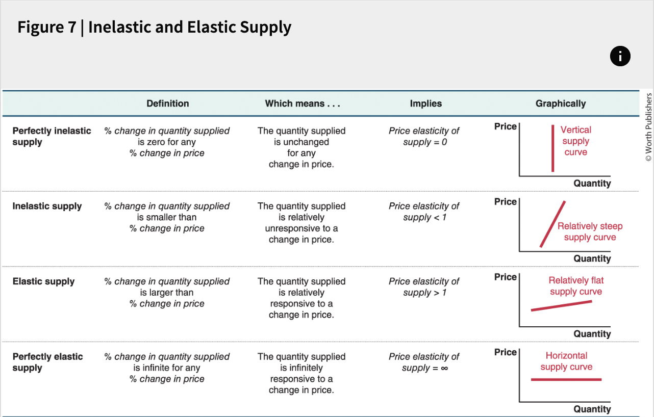
Measures responsiveness of quantity supplied to a price change
Calculation:
Similar structure to demand, positive since more supply is encouraged by higher prices
Example:
Price of services increases, will suppliers increase quantity supplied?
Determinants:
How easily can producers adjust production levels?
Flexibility relates to the ability of the business to ramp production up or down quickly
Additional Illustrative Calculations
Example Calculation for Price Elasticity
If a tutor charges $15/hour and expects $20/hour:
Initial quantity supplied at $15: 5
New quantity supplied at $20: 8
Percentage change in price: 33.33%
Percentage change in quantity: 60%
Final Remarks
Emphasize taking time on exams to avoid errors
Distinguish between similar concepts clearly to prevent confusion
Conclusion
All calculations and interpretations discussed above should be memorized or clearly noted to ensure understanding before exams.
Understanding Demand
Demand is characterized as downward sloping, meaning:
As price increases, quantity demanded decreases.
The extent of this decrease can be variable (a lot or a little).
Understanding demand is crucial for business decisions, especially regarding pricing strategies. Considerations include:
Business Context:
If many substitutes exist in the market, price increases may drive consumers away, necessitating a decrease in price to attract more buyers.
Conversely, if the product is unique, raising the price may not deter customers, and revenue could increase.
Price Elasticity of Demand
The price elasticity of demand examines how quantity demanded responds to price changes:
It concentrates on the slope of the demand curve, analyzing whether it is steep or flat.
Key metric: the price elasticity of demand defines how responsive consumers are to price changes:
Results are critical when analyzing effects of pricing changes on revenue.
Types of Elasticities to be Covered:
Price Elasticity of Demand: Focus on how quantity demanded changes with price movement.
Price Elasticity of Supply: Examines production changes with price fluctuations.
Cross Price Elasticity: Measures the impact of a substitute's price change on the demand of a related product.
Income Elasticity of Demand: Assesses how demand shifts when consumer income fluctuates.
Price Elasticity of Demand - Definitions and Computation
Calculation:
Price elasticity of demand measures responsiveness as the percentage change in quantity demanded divided by the percentage change in price:
Example Calculation: If the price of t-shirts decreases by 15% and quantity demanded increases by 25%, the elasticity would be:
E_d = rac{25 ext{%}}{-15 ext{%}} = -1.67Interpretation:
An elasticity of -1.67 indicates that for a 1% increase in price, quantity demanded decreases by 1.67%. Thus, demand is elastic.
If elasticity is less than 1 (e.g., 0.3), it indicates inelastic demand.
Categories of Demand Elasticity
Responsive Demand: When elasticity (absolute value) exceeds 1, indicating consumers respond significantly to price changes.
Example: Luxury goods or easily substituted items like specific brands.
Inelastic Demand: When elasticity is less than 1, indicating minimal response to price increases.
Example: Essential goods like gas or medications that consumers must purchase regardless of price changes.
Perfectly Inelastic Demand: Denotes a situation where quantity demanded remains constant despite price changes (e.g., addictive substances).
Perfectly Elastic Demand: Represents products that have almost infinite substitutes, leading to zero consumption if prices rise.
Application of Price Elasticity in Real-World Scenarios
Market Example: Consider the impact of biking popularity on the market for electric vehicles (EVs):
Biking becoming more popular decreases the quantity demanded for EVs, leading to a leftward shift in the demand curve for EVs.
Result: Decreased price and quantity traded in the market for EVs.
Elasticity and Business Strategies
Understanding elasticity helps businesses decide:
Whether to raise or lower prices based on demand responsiveness to maximize revenue.
Higher prices could lead to lower total revenue if demand is elastic; thus, reducing prices may attract more customers.
Relevant Examples and Case Discussions
Consider the case of university tuition fees increasing by 10%, resulting in a 3% decrease in enrollment leads to a calculated elasticity of demand:
E_d = rac{3 ext{%}}{10 ext{%}} = 0.3, indicating demand is inelastic, as enrollment does not significantly drop with tuition hikes.
A case study on the New York City Tennis Courts:
Price increase from $100 to $200 may decrease demand from 12,000 to 7,000 permits, calculated via the midpoint formula, illustrating how elasticity can affect pricing in niche markets.
Summary of Key Points on Elasticity
Inelastic Demand: A direct relationship where necessity items or products with fewer substitutes lead to less responsive consumer behavior.
Elastic Demand: Consumers actively seek substitutes or are price-sensitive, responsive to price changes with diverse options available.
Elasticity Implications: Affects overall market dynamics, impacting pricing, revenue management, and strategic business decisions.
Conclusion
Elasticity is crucial for effective market strategy and understanding consumer behavior of goods, especially in terms of necessities versus luxuries and the existence of substitutes.
Practical applications of elasticity concepts extend to various real-world economic scenarios and business strategies, implicating how prices can and should adjust based on consumer response to maximize revenue and market presence.
Class will reconvene to continue discussions and case explorations on Thursday for further insights into elasticity and associated real-world applications.
In-person: Sunday, October 26, from 7–9 p.m. in McCain Auditorium 1.
Our wonderful TAs, Liam and Allie, will go over practice problems and answer your questions.Online: Monday, October 27, from 7–9 p.m., for any last-minute questions.
Chapter Six: Government Intervention
Concept Overview:
Examines the implications of government intervention in the economy
Efficiency vs. Equity:
Market assumptions lead to efficient outcomes under perfect competition; however, they might not ensure equity.
Need for collective decisions on societal needs (e.g., food, housing) since markets do not address these directly, primarily focusing on individual preferences and purchasing power.
Government Interventions Discussed
Taxation:
Can be used to deter negative health behaviors (e.g., smoking taxes to reduce lung cancer).
Provide revenue for public goods and services (roads, schools, hospitals).
Taxes can come from income, goods (luxury, groceries), etc.
Minimum Wage Legislation:
Sets a legal floor on income for workers, yet may cause market distortions and potential trade-offs (protecting some while creating challenges for others).
Housing Market Interventions:
Rent controls as a form of equity intervention to make housing affordable but may lead to shortages or market dissatisfaction from landlords.
Elasticities and Their Implications
Cross Price Elasticity
Definition:
Measures how the quantity demanded of one good (Good B) responds to a change in the price of another good (Good A).
Example Calculation:
If the price of Good A decreases by 2% and the quantity demanded increases by 14%, while Good B’s demand increases by 17%, the formula for cross-price elasticity is given by:
Using the numbers provided, the resulting elasticity indicates whether goods are substitutes (positive elasticity) or complements (negative elasticity).
Price Elasticity of Supply
Definition:
Indicates how the quantity supplied of a good responds to price changes.
Example:
When the price of pens rises from $1.90 to $2.20, and production increases from 38 to 42 million units, one would calculate the price elasticity of supply using the formula:
Demand Analysis in Contexts
Substitutes vs. Complements
Natural Gas and Heating Oil:
Examining two goods in the housing heating market where technological advancements increase the supply of natural gas.
Resulting lower prices and increased consumption of natural gas, leading to a decrease in demand for heating oil, indicating they are substitutes.
Demand Elasticities:
Demand may behave differently based on market characteristics, with inelastic demand for grains globally contrasted against potentially more elastic demand for local grains (Kansas).
Revenue implications differ based on overall market conditions and the elasticity of demand present in each scenario.
Overview of Tax and Consumption Trends Example
Discussion focused on soda tax implemented to address health issues related to sugary beverages.
Increase in Demand for Sugary Drinks
Data on Increased Consumption:
Energy drinks: +638%
Sweetened coffees: +579%
Flavored water: +527%
Drinkable yogurt: +283%
Health Concerns:
High sugar content in beverages linked to health risks such as diabetes, heart disease, etc.
Sugary drinks contribute significantly to these risks.
Implementation of Soda Tax
Example of Legislation:
Region: Newfoundland and Labrador, Canada
Date Implemented: February 2022
Tax Rate: 20¢ per liter on sugary drinks.
Objectives of the Tax:
Generate revenue for the government.
Discourage consumption of sugary drinks by increasing their price.
Higher prices lead to lower consumption rates.
Projections for Health Issues
Long-term Health Implications (Next 25 Years in Canada):
More than 1 million Canadians expected to become overweight.
More than 3 million expected to become obese.
Additional health issues projected:
1 million cases of diabetes (particularly type 2 diabetes).
300,000 Canadians with heart disease.
100,000 cases of cancer.
40,000 cases of strokes.
Broader Implications of Soda Tax
Market Freedom vs. Health Costs:
Market dynamics advocate for individual choice in consumption but ignore health costs borne by individuals and society.
Social costs like healthcare fall on society if individuals develop health issues related to sugary drink consumption.
Impact on Public Opinion:
Tax repealed in 2025 due to public opposition to higher prices.
Similar opposition noted in New York City where low-income groups rejected soda tax intended to protect their health.
Discussion on Taxation Strategies
Question of Tax Targeting:
Should the government impose taxes on groceries or meals at fancy restaurants?
Discussion led to considerations of equity and economic burden across different income groups.
Economic Burdens of Taxes
Definitions:
Statutory Burden: Tax legally imposed (e.g., on sellers or buyers).
Economic Burden: Actual burden of a tax, impacted by market dynamics (who ultimately pays).
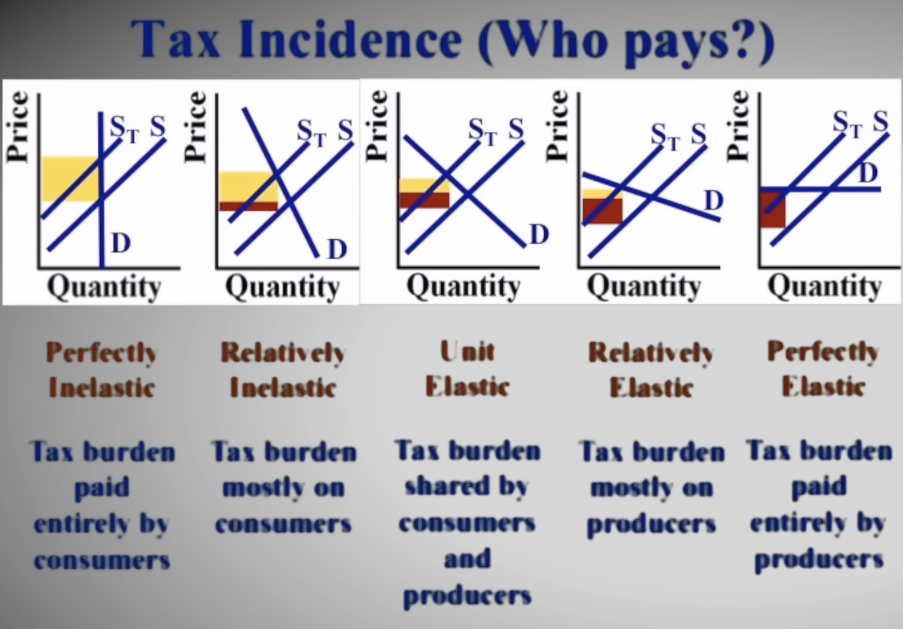
Tax Incidence: Distribution of tax burden between buyers and sellers determined by elasticity of supply and demand.
Price Dynamics of Tax Imposition
Example of Tax on Sellers:
Original price: $1.55
After imposing tax (20¢):
Price buyers pay (PB) increases
Price sellers receive (PS) decreases.
Resulting Consumer Impact:
Slight increase in price leads to decrease in consumption, aligning with the goal of the tax.
Tax Incidence Calculations
Calculation Example:
Initial price paid by consumers ($1.55) compared to new price ($1.70).
Burden on consumers = increase of 15¢, contributing to 75% of the total burden of the tax.
Burden on sellers = decrease in revenue, retaining only 25%.
Elasticity and Tax Burden
Elastic vs. Inelastic Demand Curves:
Analyzed based on shape and responsiveness of consumers to price changes.
Impact of Elasticity on Tax Payment:
More inelastic demand means consumers bear greater burden regardless of who the tax is levied on.
Results seen in both groceries (inelastic demand) and fancy restaurants (more elastic demand).
Additional Health and Economic Policies
Examples of Tax Applications:
Cigarette taxes as a case study.
New smokers more responsive to price increases than older, addicted smokers.
Public Health versus Freedom:
Discussion centers around government intervention in personal choice versus societal health outcomes.
Conclusion
Key Takeaways:
Tax policies effectively increase price and can decrease consumption of harmful products.
Understanding market dynamics and elasticity can better inform design and implementation of such taxes to achieve desired public health outcomes.