L5 Statistical inference
1. Introduction to Statistical Inference
Statistical inference allows statisticians to make informed conclusions about a population based on a sample.
Essential concepts include normal distribution and p-values.
2. Importance of Sample Selection
2.2. Random vs Non-Random Samples
Random Samples: Preferable as they represent the population accurately.
Every individual in the population has an equal chance of being selected.
Facilitates generalization of research results to the broader population.
Non-Random Samples: May lead to biased results and less reliable conclusions.
3. The Principle of Statistical Inference
Facilitates the leap from known sample results to unknown population parameters.
The normal curve plays a crucial role in this inference process.
4. Normal Distribution
4.1 Characteristics of the Normal Curve
Mathematically defined bell-shaped distribution.
No skewness or kurtosis.
Common in many natural variables (e.g., heights, IQ scores).
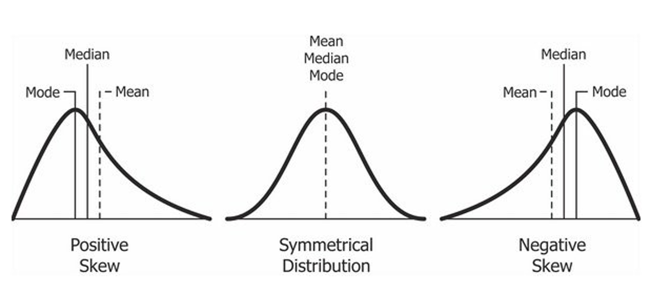
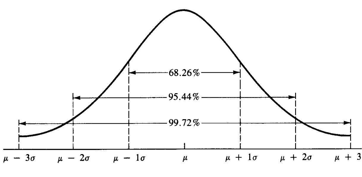
4.2 Key Features
Mean = Median.
Roughly 68.26% of observations fall within ±1 standard deviation from the mean.
Approximately 95.44% within ±2 standard deviations, and about 99.72% within ±3 standard deviations.
5. Standardization and Z-Scores
5.1 Conversion to Standard Scores
Z-scores express values in terms of standard deviations from the mean.
A z-score of 0 corresponds to the mean, while a z-score of ±1 indicates one standard deviation away.
Useful for comparing scores from different distributions.
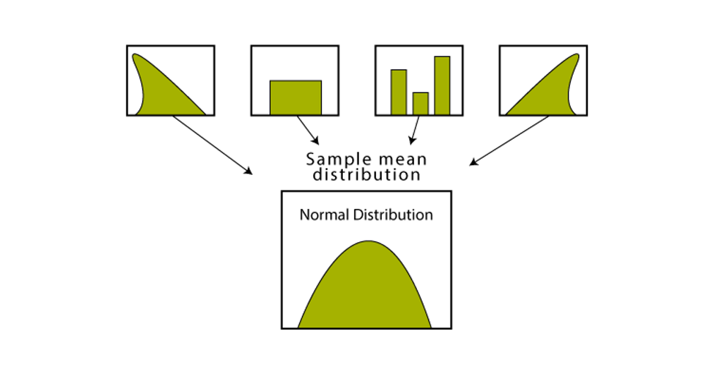
6. Central Limit Theorem (CLT)
States that sample means will be normally distributed regardless of population shape if sample size is sufficiently large.
Enables estimation of population parameters from sample means.
Standard error formula: SE = σ / √n, linking sample and population standard deviations.
7. P-Values
7.1 Understanding P-Values
A statistical measure that indicates the likelihood of results from a sample applying to the population.
Standard cut-off: p < 0.05 indicates statistical significance.
Indicates confidence level in the generalization from sample to population.
7.2 Interpretation of P-Values
Example: p = 0.01 shows 99% confidence that results are valid for the broader population.
Higher p-values suggest less confidence in generalization.
8. Confidence Intervals
Used to estimate the range of a population parameter.
A 95% confidence interval indicates there's a 95% chance the true population value falls within that range.
Example: If a favorability rating is 63% with a margin of error of ±3%, the real favorability ranges from 60% to 66%.
9. Types of Errors
9.1 Type I and Type II Errors
Type I error: Incorrectly rejecting a true null hypothesis (false positive).
Probability of finding a statistically significant result in your sample when, in fact, there is no relationship in the population.
Type II error: Failing to reject a false null hypothesis (false negative).
Probability of not finding a statistically significant result when, in fact, there is a relationship in the population.
Both types of errors have many causes, [e.g., sample size, non-random samples, measurement error, etc.]
10. Significance of Inferential Statistics in Business Analytics
Helps derive conclusions from limited data to infer insights about broader populations.
Crucial for future predictions and informed decision-making in business contexts.
11. Revision Questions
Importance of representative samples and methods to ensure representation?
Definition and significance of the normal curve in statistics?
Explanation of the central limit theorem's role in generalization?
Definition and significance of p-values?
Difference between Type I and Type II errors and factors affecting them?