Chapter 11: Consumption; Investment; Government Spending

I. Consumer Spending

• To develop the Keynesian Aggregate Expenditures model, we must understand the basic macroeconomic relationships that are the components of that model.

• The components of aggregate expenditures in a closed economy are Consumption, Investment, and Government Spending.

• Because government spending is determined by a political process and is not dependent on fundamental economic variables, we will focus in this lesson on an explanation of the determinants of consumption and investment.

• Income = Consumption + Savings

  • If income goes up then consumption will go up and savings will go up.

    Consumption is a huge fraction (more than 2/3) of total spending in the economy. ($10 trillion of the $15 trillion GDP)

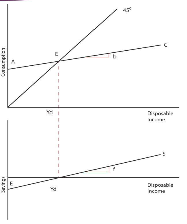
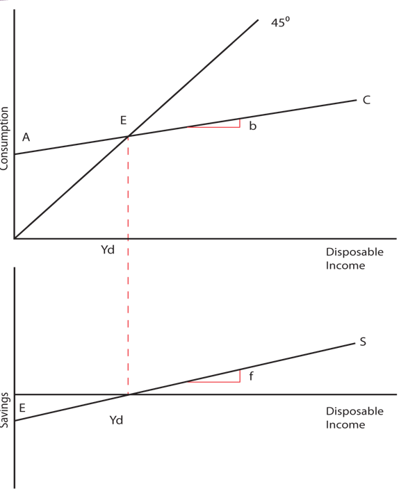
  • The graph shows consumption as a positive function of Income:

  • At the point, labeled E in our graph, savings is equal to zero. At income levels to the right of point E (like Io), savings is positive because consumption is below income, and at income levels to the left of point E (like I'), savings is negative because consumption is above income. How can savings be negative?

  • 

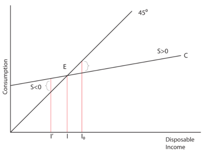
• How can savings be negative?

  • In economics we call this “dissavings.”

  • Point E is called the breakeven point because it is the point where there are no savings but there are also no dissavings.

• Consumption Function

  • The graph next demonstrates the relationship between consumption and savings.

  • The Consumption Function shows the relationship between consumption and disposable income.

  • Disposable income is that portion of your income that you have control over after you have paid your taxes.

  • To simplify, we will assume that Consumption is a linear function of Disposable Income, just as it was graphically shown here.

  • C = a + b Yd

  • In any case, “a” is the amount of consumption when disposable income is zero and it is called “autonomous consumption,” or consumption that is independent of disposable income.

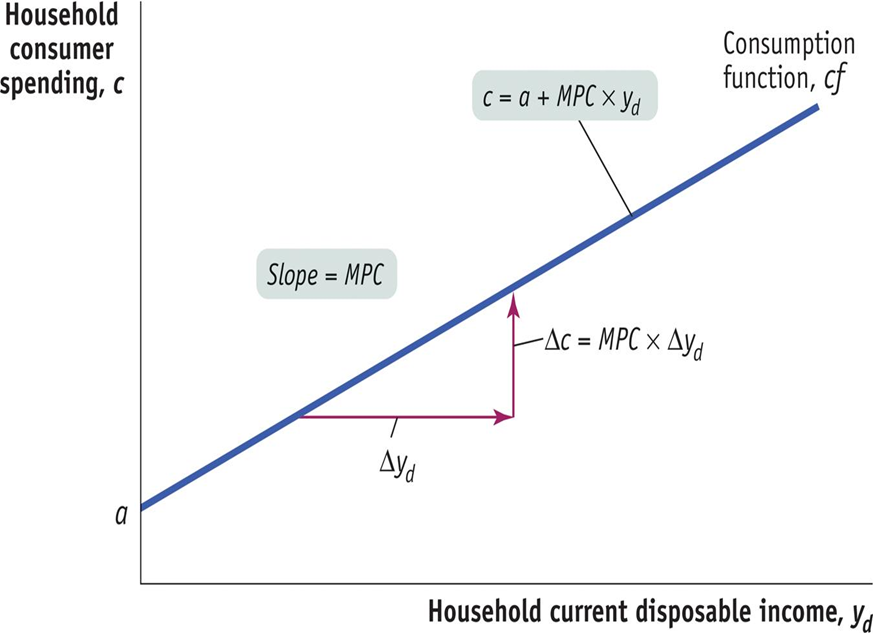
  • In the consumption function, b is called the slope. It represents the expected increase in Consumption that results from a one unit increase in Disposable Income. Also called Induced consumption in other textbooks.

    • 

• If Income is measured in dollars, you might ask the question, “How much would your Consumption increase if your Income were increased by one dollar?” The slope, b, would provide the answer to that question. It is the change in consumption resulting from a change in income.

  • Remember the idea of a slope being the rise over the run? The rise is the change in Consumption and the run is the change in Income, and you will see that this definition of b is consistent with the definition of a slope.

  • In economics, “b” is a particularly important variable because it illustrates the concept of the Marginal Propensity to Consume (MPC).

  • Average Propensity to Consume (APC): the percentage of disposable income spent, found by total consumption divided by total disposable income.

• Saving Function

  • The Savings Function shows the relationship between savings and disposable income. As with consumption, we will assume that this relationship is linear:

  • S = e + f Yd

  • In this equation the intercept is e, the autonomous level of Savings. With savings, it is quite likely that “e” will be negative, which indicates that when Disposable Income is zero, Savings on average are negative.

  • The slope of the savings function is “f,” and it represents the Marginal Propensity to Save—the increase in Savings that would be expected from any increase in Disposable Income.

  • Average propensity to save (APS): the percentage of disposable income saved, found by total saving divided by total disposable income.

    • 

I. The MPC and MPS

• Marginal Propensity to Consume (MPC)

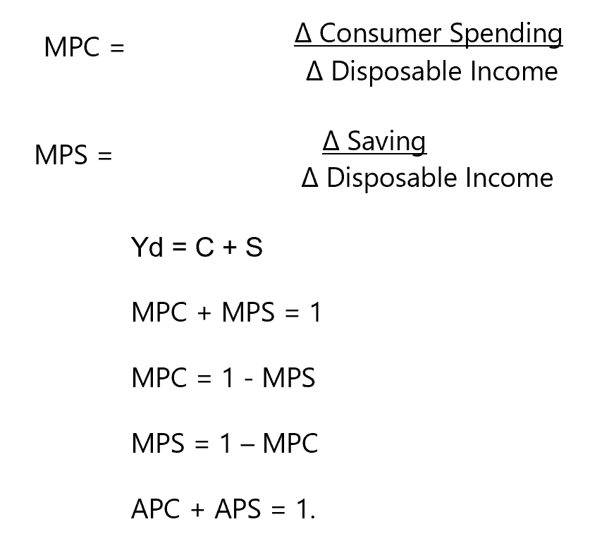
  • Yd = C + S

  • When a person gets more disposable income, Yd, he will increase both C and S.

  • MPC = (Δ Consumption/Δ Disposable Income).

  • The MPC is the amount by which consumer spending rises if current disposable income rises by $1 and is the slope of the consumption function.

• Marginal Propensity to Save (MPS)

  • MPS = (Δ Saving/Δ Disposable Income)

  • The MPS is the amount by which consumer saving rises if current disposable income rises by $1 and is the slope of the saving function.

• 

• Example:

  • 

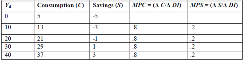
    • We can see in the table that when Yd increases by $10, C increases by $8 and S increases by $2.

      Thus the MPC = (Δ C/Δ Yd) = .8 and

      The MPS = (Δ S/Δ Yd) = .20.

      So if this household receives $1 of additional Yd, they will consume 80 cents and save 20 cents of it.

  • c = a + MPC × yd

    • 

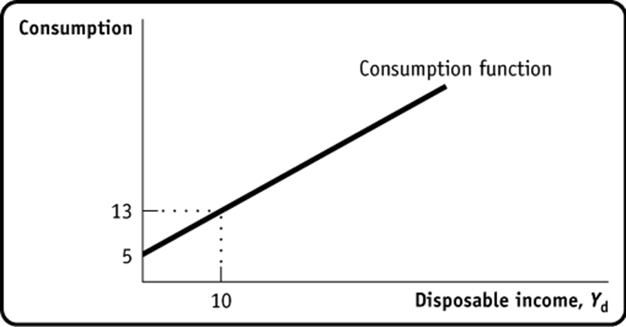
      • a: represents autonomous consumption or the vertical intercept of the function ($5).

        MPC is the marginal propensity to consume, or the slope of the function (.80).

      • c = 5 + .80Yd

• The Multiplier: An Informal Introduction

  • 

  • The Spending Multiplier

    Example: Ted is a chicken farmer in the local community.

    Suppose Ted decides to spend $1000 on some chicken coops at Anthony’s farm supply shop.

    This money now starts to be circulated around the economy.

    1. Anthony now has $1000 from the sale and spends 80% ($800) on clothes at Marcia‘s boutique.

    2. Marcia now has $800 from the sale and spends 80% ($640) to fix her car at Pat’s garage.

    3. Pat now has $640 from the sale and spends 80% ($512) at Dianna’s grocery store.

    4. Dianna now has $512 from the sale and spends 80% ($409.60) with Catherine’s catering company.

    After 5 rounds of spending, we’ve created $2,361.60, more than DOUBLE the original injection of spending. If we had continued until someone was trying to spend 80% of nothing, Ted’s initial $1000 purchase would have multiplied to a total of $5000 in income/spending

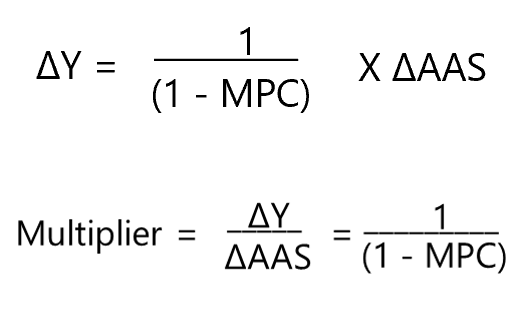
  • The Spending Multiplier

    • The spending multiplier can be shown to be equal to:

      • M = 1/(1-MPC) = 1/(1-.80) = 1/.2 = 5

    • Since MPC + MPS = 1, we can also say that M=1/MPS

      • 

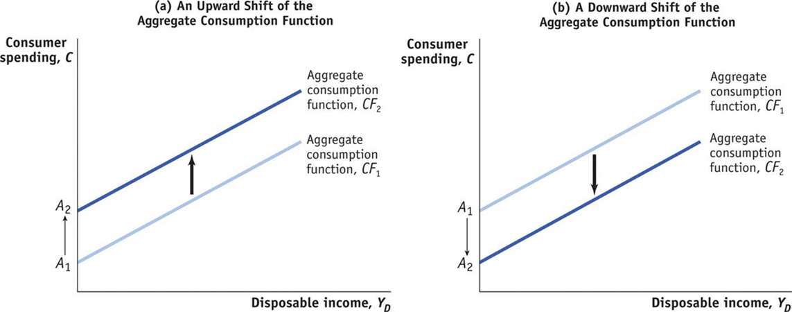
• Shifts of the Aggregate Consumption Function

  • Changes in Expected Future Disposable Income

  • Permanent Income Hypothesis

  • Changes in Aggregate Wealth

  • Life-cycle Hypothesis

    

III. Investment Spending

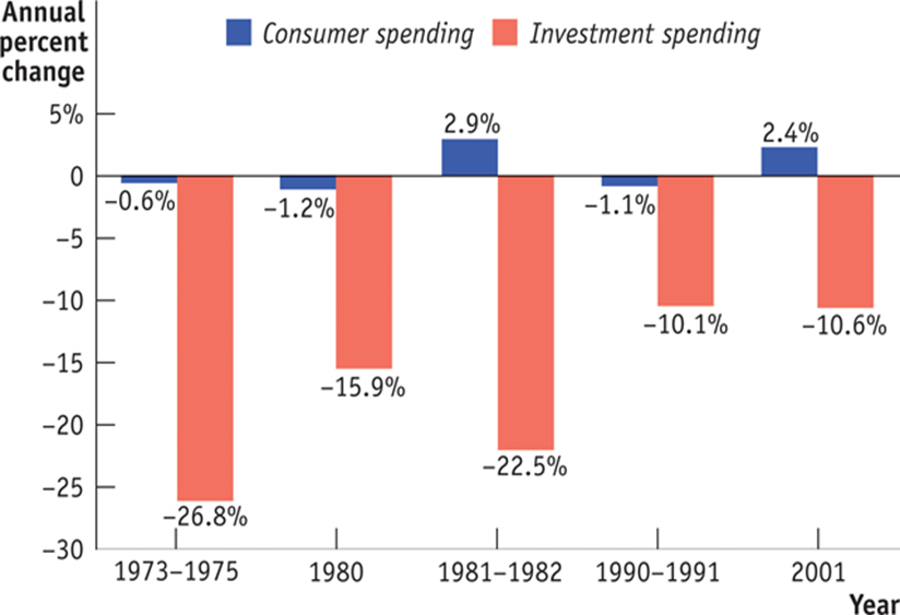
• Although consumer spending is much larger than investment spending, booms and busts in investment spending tend to drive the business cycle.

• Most recessions originate as a fall in investment spending.

  • 

• Planned Investment vs. Unplanned Investment

  • In equilibrium, planned spending must equal actual spending in the economy. The difference between planned and actual expenditure is unplanned inventory investment. ...

  • In accounting and business planning, unplanned inventory refers to the difference, positive or negative, between the inventory you need and what you actually have.

  • To calculate a business' unplanned inventory investment, subtract the inventory you need from the inventory you have. If the resulting unplanned inventory investment is greater than zero, then the business has more inventory than it needs.

• Investment: the purchase of new plant, equipment, and buildings and the additions to inventories.

  • Investment only occurs when real capital is created.

  • Investment affects both short-run and long-run economic growth.

  • Investment is a component of aggregate expenditures so when a company buys new equipment or builds a new plant/office building, it has an immediate short-run impact on the economy

  • If a company buys a new machine, that machine is going to operate, continue to produce, and will have an impact on the productive capacity of the economy for years to come. This is in contrast to consumption purchases that do not have the same impact.

  • If you buy and eat an apple today, that apple does not continue to provide consumption benefits into the future.

  • “Why do firms invest?”

    • Investment is guided by the profit motive—firms invest expecting a return on their investment.

    • Before the investment takes place, firms only know their expected rate of return. Therefore, investment almost always involves some risk.

• Determinant of investment:

  • Interest rate: the cost of borrowing money.

    • Interest rate = Interest paid/Amount borrowed.

  • Expected rate of profit.

    • Expected rate of profit = Expected profits/Money Invested.

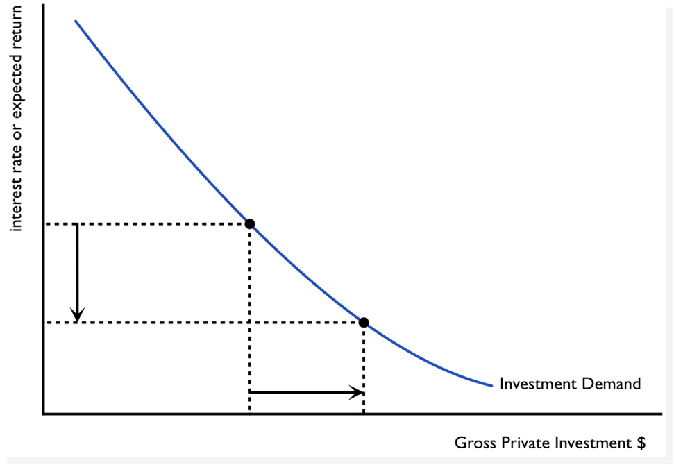
  • A decrease in the real interest rate will result in more gross private investment.

    • 

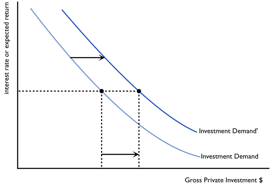
• Shifters of investment:

  • Business Taxes

  • Changes in Technology

  • Stock of Capital Goods on Hand

  • Expected Future Real GDP

  • Production Capacity

    • 

• 2. Expected rate of profit

  • = Expected profits/Money Invested

• Recall how investment is financed? Loanable Funds Market

  • Private Saving

    • Government budget surplus

    • Borrowing from the rest of the world

  • National Savings = household saving + business saving + government saving.

  • Government Savings = net taxes - government expenditure.

• Revisit Government Spending

  • Direct tax: a tax with your name written on it, such as personal income tax and social security tax, corporate income tax.

  • Indirect tax: Not tax on people but on goods or services that we purchase, such as sales tax, excise tax on tires, gasoline, movie tickets, airline tickets, cigarettes, and liquor.

  • Government budget balance = Tax revenue – Government spending