Topic 9
Principal Components and Factor Analysis
What is depression and how do we measure it? Could we simply ask someone: are you depressed (yes/no)?
The answer is no – depression is a very multifaceted concept and not everyone has the same ideas about it.
Some of these are more related to one another than others
Some are more important to the explanation of depression that others
Principle components analysis (PCA) and factor analysis (FA) are exploratory analyses that aim to map different items onto a few underlying factors that make up a construct – like depression – to best explain what this construct consists of.
PCA and FA both group items through their connection to a new compositive variable, called a component/factor
e., both are exploratory data techniques
PCA and FA both mathematically form linear composites that represent the underlying structure of the correlation matrix in terms of groups of items of correlated items whose variance is (ideally) explained by the given composite
The composite is what becomes the construct/factor
Cannot test the significance of the factors – PCA/FA are exploratory and descriptive analyses only
PCA:
Used when producing a new scale as it can maximise the variance extracted in the outcome; because all variance is included (unique, shared, and error)
Based on correlation / covariance
FA:
Can also be used when producing new scales, but is also often used to test already existing theories or scales
Also based on correlation/ covariance but excluding any unique variance.
PCA is based on the pattern of correlations among variables (the correlations matrix). For example:
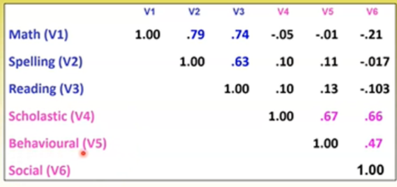
V1-3 = latent factor achievement V4-6 = latent factor competency Can see achievement items are highly correlated with one another and weakly correlated with competency items, and vice versa.
This matrix alone cannot tell us what the underlying constructs are. We need conceptually informed hypotheses to direct our interpretation of this table.
Every item needs to have an inter-item correlation of at least .30 with at least 1 other item, else it should be removed
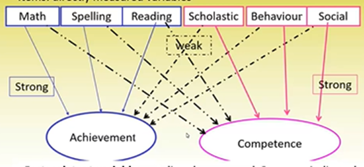
The provided items need to load onto specific latent factors (e.g., achievement and competence)
These are not directly measured: their presence is indicated by item scores
All items have a relationship with each factor, however, these correlations will likely be much weaker for the factor/s the item doesn’t load onto. For example:
Factors are formed based on the shared variance in the items included in the scale.
In PCA, all of the variance in each item is included in the analysis (unique, shared, error)
This is because PCA aims to maximise the % of variance accounted for by each of the factors extracted
FA uses only the shared and error variance
Communality: the percentage of variance in the individual items that is accounted for in the solution
PCA: will be 1 prior to analysis because 100% of the variance is used
FA: will be less than 1 prior to analysis because unique variance is excluded
Dimension Reduction Techniques
Data reduction techniques try to make sense of the world through grouping like characteristics and separating characteristics that are different into different groupings – called summarising
They ultimately aim to find underlying dimensions or relationships among variables that these characteristics can be grouped by
Used in the development of scales
Can summarise related groups of variables for use in other analyses
Research Questions
Research questions relating to data reduction techniques may include:
Is there an underlying structure linking subsets of items from a scale?
What is the nature of the latent variables underlying this construct?
Latent variables: variables not being directly measured (like achievement or competency in this example – the factors/constructs)
Conceptual Basis – the Extraction Process
The extraction process is the process of teasing apart the underlying factors that a scale taps into. This is based on eigenvectors, which are formed to extract to shared variance in the solution – this uses a stepwise process.
The initial factor extracted will extract all shared variance between items that it can – maximises variance explained
Anything leftover is the residual
This same process occurs for any other factors but their eigenvalues will be smaller
Eigenvectors: mathematically compute the principal components from the correlations matrix
Eigenvalues: the proportion of variance extracted by each eigenvector
The total initial eigenvalue will equal the total number of items (e.g., six items = eigenvalue of six), but we will want to summarise this into a smaller number
For example:
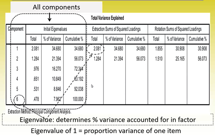
Can see the initial eigenvalues add up to 6 for the 6 items included in the scale, and this is summarised by SPSS automatically
How to Determine the Number of Factors to Expect in PCA/FA
This is a controversial topic!
1st strategy is using statistics only
All items with an eigenvalue > 1 should be extracted as a factor
Use a scree plot (or parallel analysis – a bit like bootstrapping)
Scree Plot:
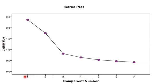
Look for the shoulder of the curve: the point in which the distance between the size of the eigenvalues becomes reduced.
Anything before this point can be extracted as a factor
Parallel Analysis:
Cannot be conducted directly in SPSS
Parallel analysis puts the number of items, the sample size, and the technique (PCA or FA). From this, 1000 samples are generated to produce eigenvalues for all components. This provides:
Average eigenvalues for each component
95% percentile eigenvalues for each component – this is preferred over the average eigenvalues
Can compare SPSS’s eigenvalue with the parallel analysis eigenvalue; if ours is larger, the factor is viable and can be extracted
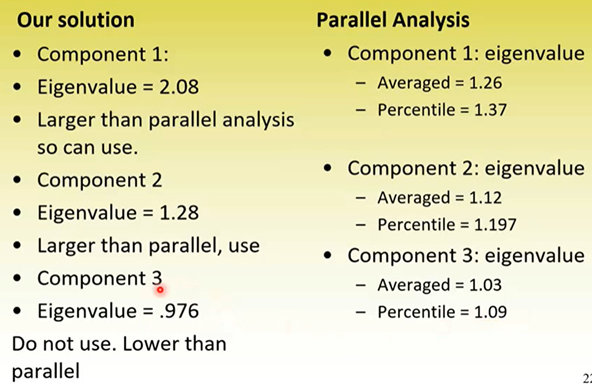
Could extract components 1 and 2 but wouldn’t extract component 3 Looking back to the provided example:
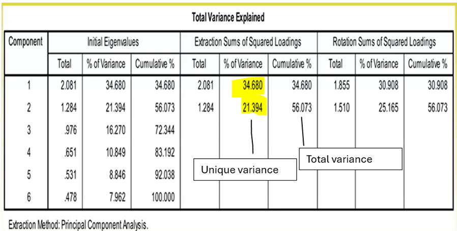
Can see the 2-factor solution produced by SPSS is consistent with the scree plot and parallel analysis
This is neat – it doesn’t always work out like this
2nd strategy is using a self-determined method
Based on theory and concepts in the research area
Researcher determines number of components extracted based on this
The preferred option
The aim of any solution is to maximise the variance accounted for by each component.
Components altogether should account for 25% of variance at least
Wont be able to account for 100% because we are trying to summarise – by the nature of this, some variance is lost
Each component should be conceptually meaningful with at least 4 factors with factor loadings at least .30
Better solutions may use a cutoff of .40
For example: the total variance explained table explains initially how variance is accounted for, where each item is considered a component, and reduces this down (in this instance to 3 components)
Initially they added up to account for 100%
The process of extraction/ summarisation reduces this – but this example is still quite good
Anything over 65% is considered great
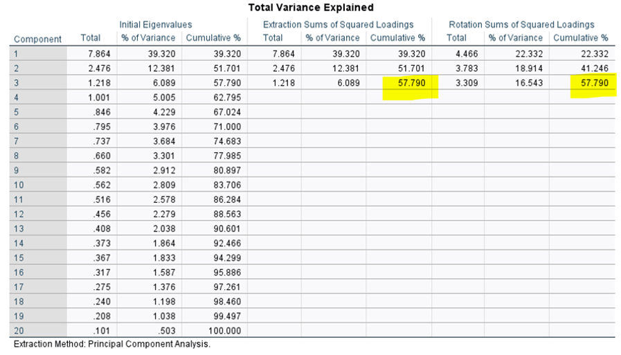
This also exhibits how with any rotation, the overall variance explained doesn’t change, but the way it is partitioned between components changes.
Interpreting Factors Using Factor Loading
Factor Loadings: the correlations between each item and the component
Range between +/- 1
Interpreted as a correlation
The larger the factor loading, the more likely that item loads onto that factor
Each item has a factor loading for each component. We want each item to have a high loading on one factor at a time only.
Because this produces a solution with independent solutions
Important because with PCA and FA we are trying to explain the different components of a multidimensional construct
We need at least 100 participants in a PCA or FA. where n =/> 100, factor loadings:
.30-.39 minimum (accounting for 10% variance)
.40-.49: stronger/ more robust (16% variance)
.50-.59: practically significant (> 25% variance)
.70: very strong effect, this item is very important
Its unusual to have loadings over .80
Linear Combinations
Each factor is made up of the sum of all items on the scale. These produce a linear composite that is weighted by the item factor loading to reflect how strong the relationship is between each item and the factor
Ability factor = .8math + .7reading + .7spelling + .1scholastic + .01behavioural + .2social
Competence factor = .01math + .1reading + .02spelling + .7scholastic + .6behavioural + .65social
Can see that ability items have higher loadings onto the ability factor, and competency items have higher loadings on the competency factor
This is like an ideal scenario – similar items have high associations with one factor and low associations with the other factor/s
Factor Component Matrix
Items Components
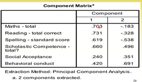
What we want are:
High factor loadings for factor 1 on the ability items
High factor loadings for factor 2 on the competency items
Can see quite a few of these items have high cross-loadings. Why does this happen?
Mathematically, the initial components matrix will try to maximise the variance accounted for by factor 1 – trying to generate a general component
So factor 1 has a very high eigenvalue
It will have relatively high loadings on as many items as possible
Therefore, the initial component matrix is not interpretable in the way we want, because there is no good way to separate the independent components
We can apply a factor rotation to deal with this: mathematically reorganises the way the variance is assigned to the different components by moving the factors themselves.
Component Factor Rotations
There are two types of rotations:
Independent/ orthogonal rotations: used when components are independent of one another
Correlated/ non-independent/ oblique rotation: used when components can be correlated with one another
Factors can be represented in 2D space.
Components initially represented perpendicular to one another (separated at the origin by a 90 degree angle)
Means they are independent
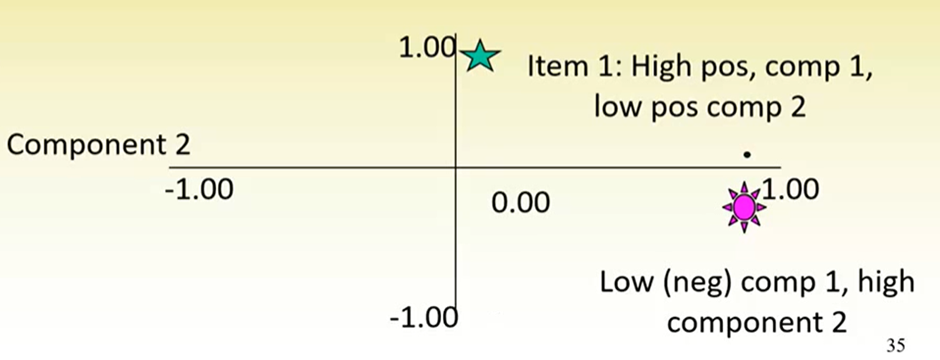
Here, 1 and 2 make up a good solution because factor 1 items load highly onto factor 1, and very weakly onto factor 2, and vice versa for factor 2 items.
Where items don’t load this nicely, we can apply a rotation to separate items more on components 1 and 2.
Unrotated Example:
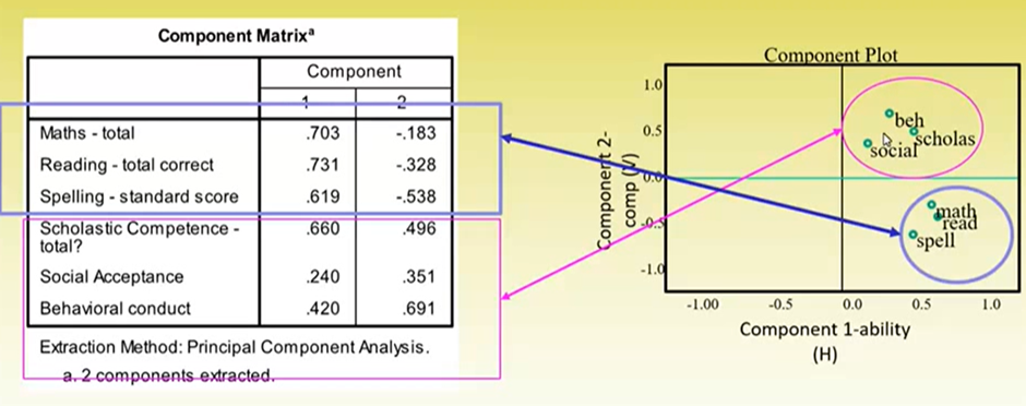
Orthogonal / Independent Rotations
For this example, we can apply an orthogonal / varimax rotation.
Maintains the independence of components
Items stay in place, it’s the components that move
Example of Orthogonal Rotation:
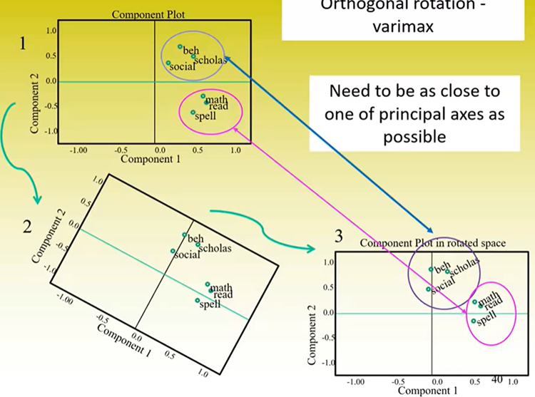
Overall, the aim is to maximise the factor loadings on the relevant component and the separation between the different groups of items
Comparing unrotated and rotated component matrices:
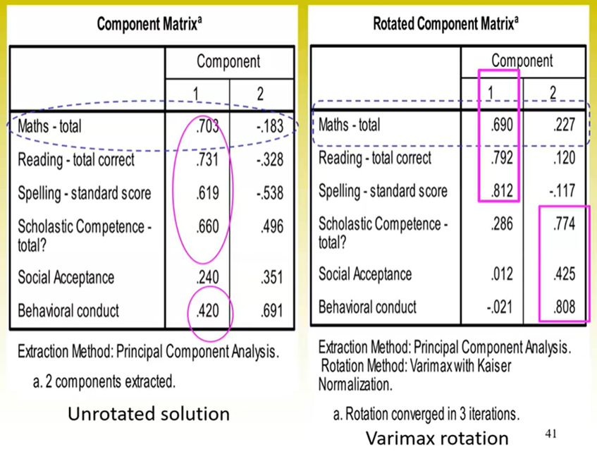
Can see rotations tend to solve a lot of the major problems we encounter with the unrotated solution.
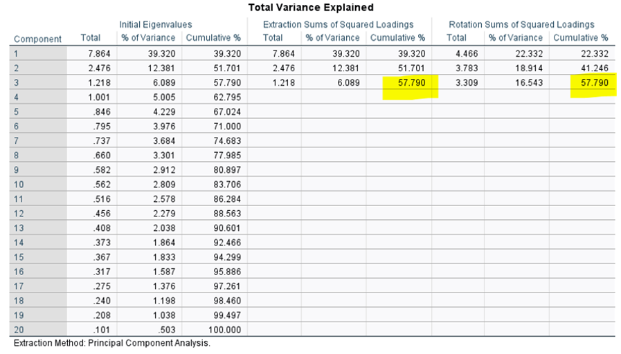
Can see here the percentage of variance accounted for by each component evens out in the rotated solution.
The eigenvalue decreases slightly for factor 1 (the general factor) and some of this is given to the subsequent factor/s
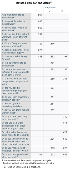
Here, there are several items that have cross-loadings with 2-3 items. Even with the rotation, this solution isn’t perfect. One way we could deal with this is by removing some items (e.g., the ones that have cross-loadings on 3 items)
How this Influences Variance Extracted
What we want to know for each item is how much variance in them is explained by the solution, i.e., how much they contribute to the solution.
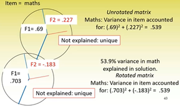
Can see when a rotation is applied, the total variance accounted for doesn’t change, but the way it is divided between factors does.
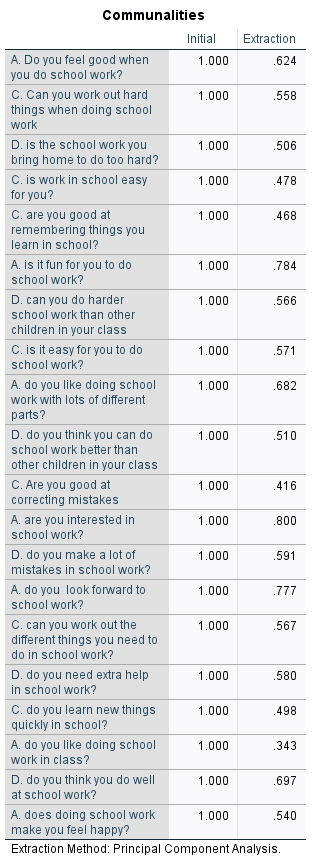
This example tells us how well the 3-factor solution explains variance in responses for each item.
How well can we predict peoples responses when we use the 3-factor solution
Most of these are pretty good
Below .4: consider whether it is worth keeping
Below .1: remove
Naming and Describing Components/Factors
The naming of factors has a number of rules:
If replicating someone else’s solution, use the same names for factors being replicated
If changing them: it needs to be clear what they correspond to in past studies
Changing makes it harder to interpret the outcome
Don’t use the name of a single item: because components should consist of a combination of items
Find something representative of that group
Interpreting the Outcome
Example:
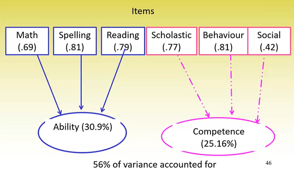
This is a robust solution because of the overall variance accounted for
Example:
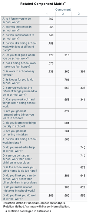
This is not a robust soliton because of the high cross-loadings.
Could remove some items
Could also try an oblique solution to see if this changes things