Digital Math.

- Foundations: Algebra

Lesson 1: Solving linear equations and linear inequalities

When solving linear equations, the most important thing to remember is that the equation will remain equivalent to the original equation only if we always treat both sides equally: whenever we do something to one side, we must do the exact same thing to the other side.

When solving linear inequalities:

• If the coefficient of x  is positive, the inequality sign maintains its direction when we divide by the coefficient to isolate x.

• If the coefficient of x  is negative, we must reverse the direction of the inequality sign when we divide by the coefficient to isolate x.

When determining the number of solutions for a linear equation:

• If the equation can be rewritten in the form x=a, where a  is a constant, then that equation has one solution.

• If the variable can be eliminated from the equation, and what remains is the equation a=b, where a  and b are different constants, then the equation has no solution.

• If the equation can be rewritten in the form x=x, then the equation has infinitely many solutions. (No matter what the value of x  is, it will always equal itself!)

Lesson 2+3+4: Linear equation and relationship word problems, graphs of linear equations and functions.

slope = change in y / change in x = (y2-y1) / (x2-x1)

The slope-intercept form of a linear equation, y=mx+b, tells us both the slope and the y-intercept of the line:

• The slope is equal to m.

• The y-intercept is equal to b.

We can write the equation of a line as long as we know either of the following:

• The slope of the line and a point on the line

• Two points on the line.

Parallel lines in the xy-plane have the same slope.

Perpendicular lines in the xy-plane have slopes that are negative reciprocals of each other.

Lesson 5: Solving systems of linear equations

To determine the number of solutions a system of linear equations has using the slope-intercept form, y=mx+b:

1. Rewrite both equations in slope-intercept form.

2. Compare the m- and b-values of the equations to determine the number of solutions.

3. If the two equations have different m-values, then the system has one solution.

4. If the two equations have the same m-value but different b-values, then the system has no solution.

5. If the two equations have both the same m-value and the same b-value, then the system has infinitely many solutions.

Lesson 6: Systems of linear equations word problems

Word problems that require us to write systems of linear equations have two unknown quantities and two different ways to relate them.

This means we need to write two linear equations, and each contains the two unknowns as variables. The Understanding Linear Relationships lesson details how to translate verbal descriptions into equations.

After we write the equations, we can solve the system using our preferred method(s) for solving systems of linear equations covered in the Solving Systems of linear equations lesson.

To solve a system of linear equations word problem:

1. Select variables to represent the unknown quantities.

2. Using the given information, write a system of two linear equations relating the two variables.

3. Solve the system of linear equations using either substitution or elimination. Linear inequality word problems

Lesson 7: Linear inequality word problems

Lesson 8: Graphs of linear systems and inequalities

When a system of linear equations is graphed, the solution appears where the lines intersect.

When we have linear inequalities in slope-intercept form:

• If y is greater than mx+b, shade above the line.

• If y is less than mx+b, shade below the line.

In slope-intercept form, inequalities with...

• Greater than (>) or less than (<) signs do not include points on the line in the solution set. We use a dashed line to show that the points on the line are not included.

• Greater than or equal to (>=) or less than or equal to (<=) signs do include points on the line in the solution set. We use a solid line to show that points on the line are included.

- Foundations: Problem-solving and data analysis

Lesson 1: Ratios, rates, and proportions

A ratio is a comparison of two quantities. The ratio of a to b can be expressed as a:b or a/b.

A proportion is an equality of two ratios. We write proportions to help us find equivalent ratios and solve for unknown quantities.

A rate is the quotient of a ratio where the quantities have different units.

Rates are used to describe how quantities change. Common rates include speed (distance/time) and unit price (total price/units purchased).

Lesson 2: Unit conversion

On the SAT, the relationships between units will be provided to you in the form of an equivalency (e.g., 1 foot = 12 inches).

It's useful to think of this equivalency as a ratio (e.g., 1 foot/12 inches ). You'll then multiply the initial measurement by that ratio to convert from one unit to the other.

Note: It's important to remember that every unit (besides the unit you're looking for) should appear once in the numerator and once in the denominator. That way, all other units can be canceled out!

Lesson 3: Percentages

Percent means parts per hundred.

 p% = p / 100

A shortcut for converting percentages to decimals is to remove the % symbol and move the decimal point left 2 places.

When translating word problems:

• "what" means x

• "is" means =

• "of" means multiplied by

• "percent" means divided by 100

The sum of all parts of a whole is 100%.

When calculating a percent change from an initial value to a final value:

1. Find the difference between the initial and final values.

2. Divide the difference by the initial value.

3. Convert the resulting decimal to a percentage.

% change = ( difference / initial )*100

Lesson 4: Center, spread, and shape of distributions

Center, spread, and shape of distributions are also known as summary statistics (or statistics for short). These measurements are used to concisely describe data sets.

• Center describes a typical value in a data set. The SAT covers three measures of center: mean, median, and occasionally, mode.

• Spread describes the variation of the data. Two measures of spread are range and standard deviation.

mean = sum of values/number of values

The median is the middle value when the data are ordered from least to greatest.

• If the number of values is odd, the median is the middle value.

• If the number of values is even, the median is the average of the middle values.

The mode is the most common value in a data set.

range = maximum value - minimum value

Standard deviation measures the typical spread from the mean.

Lesson 5: Data representations

Aside from tables, the two most common data representation types on the SAT are bar graphs and line graphs.

On a bar graph, the sizes of the bars are related to the size of the quantities: the larger a quantity is, the taller or longer the bar representing it is.

Dot plots use dots to represent the frequency with which particular values occur. Dot plots are usually used for low, easily countable frequencies because it's impractical to draw or count many dots.

Histograms use bars to represent the frequency at which a range of values occurs. Histograms are useful because it's often impractical to list every possible value independently.

Line graphs usually show how quantities change over time.

key phrases of drawing line graphs based on verbal descriptions:

Lesson 6: Scatterplots

A scatterplot displays data about two variables as a set of points in the  -plane. Each axis of the plane usually represents a variable in a real-world scenario.

While each point in a scatterplot represents a specific observation, the line of best fit describes the general trend based on all of the points.

We can also interpret the slope and y-intercept of the line of best fit the same way we interpret line graphs:

• The slope represents a constant rate of change.

• The y-intercept represents an initial value.

When making predictions based on scatterplots, always use the line of best fit instead of individual data points.

If the prediction lies within the part of the xy-plane shown, it must lie on the line of best fit.

If the prediction lies beyond the part of the xy-plane shown, we can either extend the line of best fit or use its equation to find the prediction.

For linear functions in the form f(x)=mx+b :

• Sketch a line that fits the data and approximate its slope.

• The value of m should match the slope. Make sure to pay attention to the signs!

• Approximate the y-intercept of the function that best fits the data. Make sure the constant term b matches the y-intercept.

For quadratic functions in the form f(x)=ax²+bx+c :

• Sketch a parabola and approximately fit the data.

• If the parabola opens upward, a should be positive. If the parabola opens downward, a should be negative.

• Approximate the y-intercept of the function that best fits the data. Make sure the constant term c matches the y-intercept.

Lesson 7: Linear and exponential growth

When we're given a table of (x, y) values, for a given change in  :

• If the change in y can be represented by repeatedly adding the same value, then the relationship is best modeled by a linear equation.

• If the change in y can be represented by repeatedly multiplying by the same value, then the relationship is best modeled by an exponential equation.

Using y=mx+b to represent a linear equation:

• m is the number repeatedly added, the rate of change, or the slope of the line when the equation is graphed in the xy-plane.

• b is the initial value, or the y-intercept of the line when the equation is graphed in the xy-plane.

Using y=a(b)^x to represent an exponential equation:

• b is the number repeatedly multiplied, or the common factor or common ratio.

• a is the initial value, or the y-intercept of the curve when the equation is graphed in the xy-plane.

The table below lists some common phrases in linear and exponential growth problems and how to interpret them.

Note: c is a constant in the phrases.

Lesson 8: Probability and relative frequency

Once we correctly identify the values we're looking for in a problem, the rest of the problem is basically dividing two values to find a fraction, percentage, or probability.

Note: While probabilities and relative frequencies are different concepts, we perform the same calculations for them.

Note: missing value questions appear very rarely on the test.

Just as we can calculate a probability or relative frequency using the values in two-way frequency tables, we can calculate missing values in a table when given a probability or relative frequency.

Some two-way frequency tables do not provide the totals for us. For these tables, it's helpful to add a row and a column for the totals.

Lesson 9: Data inferences

estimate = sample proportion * population

range = estimate ± margin of error

The larger the sample size is, the smaller the margin of error will be.

Lesson 10: Evaluating Statistical Claims

We can draw conclusions about only the population from which the random sample was selected.

To understand the conclusions we can draw from controlled experiments, we must first understand the difference between correlation and causation.

• Correlation means there is a relationship or pattern between the values of two variables.

• Causation means that one event causes another event to occur.

- Foundations: Advanced math

Lesson 1: Factoring quadratic and polynomial expressions

Square of sum:  a²+2ab+b² = (a+b)²

Square of difference:  a²-2ab+b² = (a-b)²

Difference of squares:  a² - b² = (a+b)(a-b)

There are more factoring formulas:

1. (x+a)(x+b) = x²+(a+b)x+ab

2. (a+b)³ = a³+ b³+ 3ab(a+b)

3. (a-b)³ = a³- b³- 3ab(a-b)

4. (a+b+c)² = a²+b²+c²+2ab+2bc+2ca

5. x³+y³+z³-3xyz = (x+y+z)(x²+y²+z²-xy-yz-xz)

6. x³+y³ = (x+y)(x²-xy+y²)

7. x³-y³ = (x-y)(x²+xy+y²)

Lesson 2: Radicals and rational exponents

Adding and subtracting exponential expressions:

axⁿ ± bxⁿ = (a±b)xⁿ

Multiplying and dividing exponential expressions:

(ax^m)*(bxⁿ) = ab*x^m+n

(ax^m)/(bxⁿ) = a/b*x^m-n

(xⁿ)*(yⁿ) = (xy)ⁿ

(xⁿ)/(yⁿ) = (x/y)ⁿ

Raising an exponential expression to an exponent and change of base:

(ax^m)ⁿ = (aⁿ)(x^m*n)

(a^b)ⁿ = a^b*n

Negative exponent:

x^-n = 1/(xⁿ)

Zero exponent:

x⁰ = 1, x ≠ 0

All of the rules that apply to exponential expressions with integer exponents also apply to exponential expressions with fractional exponents.

Lesson 3: Operations with polynomials

The mnemonic FOIL for multiplying two binomials:

1. Multiply the First terms

2. Multiply the Outer terms

3. Multiply the Inner terms

4. Multiply the Last terms

(axⁿ)*(bxⁿ) = ab*x^m+n

(a^b)ⁿ= a^b*n

Lesson 4: Operations with rational expressions:

When multiplying two rational expressions:

(a/b) * (c/d) = ac / bd

When dividing two expressions, recall that dividing by a fraction is equivalent to multiplying by that fraction's reciprocal:

(a/b) / (c/d) = a/b * d/c = ad / bc

When adding or subtracting two rational expressions with unlike denominators:

Remember that you can only add and subtract the numerators of the rational expressions if the expressions have a common denominator!

We can represent any rational expression as a(x)/b(x), where a and b are polynomial expressions in terms of x.

When dividing a and b, we can find quotient polynomial q and remainder polynomial r such that:

a(x)/b(x) = q(x) + r(x)/b(x)

Where the degree of r is less than the degree of b. Since b is usually a first-degree polynomial (ax+b), r is usually a constant.

Lesson 5: Nonlinear functions

A function takes an input and produces an output. In function notation, f(x), f is the name of the function, x is the input variable and f(x) is the output.

The input of a function can be a numeric value (exempli gratia., f(2)), an expression (e.g., f(x+1)), or even another function (e.g., f(g(x))). Functions can also be based on other functions.

Lesson 6: Isolating quantities

Isolating quantities is similar to solving equations. However, instead of ending up with a variable equal to a constant, we end up with a variable equal to an expression containing other variables.

Lesson 7: Solving quadratic equations

For ax² + bx + c = 0

• If b² - 4ac > 0, then the equation has 2 unique real solutions.

• If b² - 4ac = 0, then the equation has 1 unique real solution.

• If b² - 4ac < 0, then the equation has no real solution.

Lesson 8: Linear and quadratic systems

Linear and quadratic systems are systems of equations with one linear equation and one quadratic equation (exempli gratia, y=x²-1).

A linear and quadratic system can be represented by a line and a parabola in the xy-plane. Each intersection of the line and the parabola represents a solution to the system.

A line and a parabola can intersect zero, one, or two times, which means a linear and quadratic system can have zero, one, or two solutions.

To solve a linear and quadratic system:

1. Isolate one of the two variables in one of the equations. In most cases, isolating y is easier.

2. Substitute the expression that is equal to the isolated variable from (1) into the other equation. This should result in a quadratic equation with only one variable.

3. Solve the resulting quadratic equation to find the x-value(s) of the solution(s).

4. Substitute the x-value(s) into either equation to calculate the corresponding y-values.

Lesson 9: Radical, rational, and absolute value equations

Radical equations are equations in which variables appear under radical symbols.

Rational equations are equations in which variables can be found in the denominators of rational expressions.

Absolute value equations are equations in which variables appear within vertical bars.

The radical operator calculates only the positive square root. If a solution leads to equating the square root of a number to a negative number, then that solution is extraneous.

We cannot divide by 0. If a solution leads to division by 0, then that solution is extraneous.

For the absolute value equation, rewrite the equation as the following linear equations and solve them.

• ax+b=c

• ax+b=-c

Both solutions are solutions to the absolute value equation.

Lesson 10: Quadratic and exponential word problems

Population growth and decline:

The exponential function P for population looks like the following:

P(t)= P₀r^t

Where:

• t is the input variable representing the number of time periods elapsed.

• P₀ is the initial population, or the population when t=0.

• r describes how the population is changing.

If r>1, then the population is growing. If 0<r<1, then the population is declining.

Compounding interest:

The exponential function P for an amount of money accruing compounding interest looks like the following:

P(t)= P₀(1+r)^t

Where:

• t is the input variable representing the number of time periods elapsed.

• P₀ is the initial amount of money, or the amount of money before any interest is accrued.

• r is the interest rate applied for each time period expressed as a decimal.

Note: there is a more complex version of the formula in which the interest can be applied multiple times within a single time period (for example, an annual interest rate with monthly interest calculations).

Functions modeling these topics typically look like f(t)=a(b)^t, where a is the initial value, b describes the change, and t is the variable representing time.

• Tip: If converting the variable from a larger time unit to a smaller time unit, we need to make the exponent smaller. For example, when converting from years to months, we divide the variable representing the number of months by 12.

• Tip: If converting the variable from a smaller time unit to a larger time unit, we need to make the exponent larger. For example, when converting from months to years, we multiply the variable representing the number of years by 12.

• Verify that the two expressions give us the same values when evaluated using equivalent amounts of time, e.g., 1 year and 12 months, 2 years and 24 months, etc.

Lesson 11: Quadratic graphs

Forms of quadratic equations:

Standard form: A parabola with the equation y=ax² + bx + c has its y-intercept located at (0, c).

Factored form: A parabola with the equation y=a(x-b)(x-c) has its x-intercept(s) located at (b, 0) and (c, 0).

Vertex form: A parabola with the equation y=a(x-h)² + k has its vertex located at (h, k).

When we’re given a quadratic function, we can rewrite the function according to the features we want to display:

• y-intercept: standard form

• x-intercept(s): factored form

• vertex: vertex form

Transformations:

If the graph of y=f(x) is graphed in the xy-plane and c is a positive constant:

• The graph of y=f(x-c) is the graph of f(x) shifted to the right by c units.

• The graph of y=f(x+c) is the graph of f(x) shifted to the left by c units.

• The graph of y=f(x) + c is the graph of f(x) shifted up by c units.

• The graph of y=f(x) - c is the graph of f(x) shifted down by c units.

• The graph of y= -f(x) is the graph of f(x) reflected across the x-axis.

• The graph of y= f(-x) is the graph of f(x) reflected across the y-axis.

• The graph of y=c*f(x) is the graph of f(x) stretched vertically by a factor of c.

Lesson 12: Exponential graphs

For f(x) = b^x, where b is a positive real number:

• If b>1, then the slope of the graph is positive, and the graph shows exponential growth. As x increases, the value of y approaches infinity. As x decreases, the value of y approaches 0.

• If 0<b<1, then the slope of the graph is negative, and the graph shows exponential decay. In this case, as x increases, the value of y approaches 0. As x decreases, the value of y approaches infinity.

• For all values of b, the y-intercept is 1.

To shift the horizontal asymptote:

• For f(x) = b^x, the value of y approaches infinity on one end and the constant 0 on the other.

• For f(x) = b^x + d, the value of y approaches infinity on one end and d on the other.

To shift the y-intercept:

• For f(x) = b^x + d, the y-intercept is 1 + d.

• For f(x) = a*b^x, the y-intercept is a*1=a. In this form, a is also called the initial value.

• For f(x) = a*b^x + d, the y-intecept is a + d.

Lesson 13: Polynomial and other nonlinear graphs

For a polynomial function in standard form, the constant term is equal to the y-intercept.

For the highest power term axⁿ in the standard form of a polynomial function:

• If a > 0, then y ultimately approaches positive infinity as x increases.

• If a < 0, then y ultimately approaches negative infinity as x increases.

• If n is even, then the ends of the graph point in the same direction.

• If n is odd, then the ends of the graph point in different directions.

The polynomial remainder theorem states that when a polynomial function p(x) is divided by x-a, the remainder of the division is equal to p(a).

A rational function is undefined when division by 0 occurs.

-Foundations: Geometry and trigonometry

Lesson 1: Area and volume

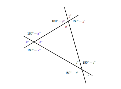
Lesson 2: Congruence, similarity, and angle relationships

• The sum of the measures in degrees of the angles of a triangle is 180.

• Similar triangles have the same shape but aren't necessarily the same size.

The corresponding side lengths of similar triangles are related by a constant ratio, which we can call k. For similar triangles ABC and XYZ, the following is true:

Lesson 3: Right triangle trigonometry

• The Pythagorean theorem: a²+b²=c²

For the right triangle ABC with angle θ shown above:

sin θ = cos (90^o - θ)

Lesson 4: Circle theorems

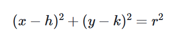
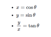
Lesson 5+6: Unit circle trigonometry and circle equations

We can describe each point (x, y) on the unit circle and the slope of any radius in terms of θ:

In the xy-plane, a circle with center (h, k) and radius r has the equation: